Chapter 9: Complex Trigonometry
Just how we have extended logarithms to the complex numbers, analytic continuation provides a natural way to extend sine and cosine to all complex inputs. Their usual power series converge for every complex input and give these extensions.
Euler’s formula, the even and odd symmetries, and the addition identities continue to hold: both sides are analytic and agree for real inputs. Through this, we will discover multiple connections between the classical trigonometric functions, their hyperbolic counterparts and complex numbers in general.
Sine and Cosine of a Complex Number
If we want to take the cosine of a complex number, we can split it up into its real and imaginary parts, and use our familiar sum of angles identity.
\[\cos(a + bi) = \cos(a)\cos(bi) - \sin(a)\sin(bi)\]
Now all we need to do is figure out what the sine and cosine of a purely imaginary number are. To do this, we will need to use our familiar Euler’s identity,
\[e^{ix} = \cos(x) + i\sin(x)\]
because it already relates complex numbers to trigonometric functions.
To leverage this formula, we will plug in an imaginary number for \(x\). Substitute \(x = iy\) with \(y\) real, so
\[e^{i(iy)} = \cos(iy) + isin(iy)\]
and by simplifying the exponent
\[e^{- y} = \cos(iy) + i\sin(iy)\]
Now we have an expression involving the cosine and sine of a complex number. In order to get one function on its own, we will consider the exponential formula with −\(x\) in place of \(x\),
\[e^{- ix} = \cos( - x) + i\sin( - x)\]
We know that \(\cos( - x) = \cos(x)\) and \(\sin( - x) = - sin(x)\), so we can simplify
\[e^{- ix} = \cos(x) - i\sin(x)\]
Plugging in \(x = iy\), we find
\[e^{y} = \cos(iy) - i\sin(iy)\]
Now we have two equations involving complex cosines and sines.
Adding them together, we can cancel the sines:
\(e^{y}\ \ \ = \cos(iy) - i\sin(iy)\)
+ \(e^{- y} = \cos(iy) + i\sin(iy)\)
\(e^{y} + e^{- y} = 2\cos(iy)\)
Isolating the cosine, we find
\[\cos(iy) = \frac{e^{y} + e^{- y}}{2}\]
The expression on the right hand side is simply one definition for hyperbolic cosine!
So we find that
\[\boxed{\cos(iy) = \cosh(y)}\]
So the cosine of an imaginary number is the hyperbolic cosine of its absolute value!
By subtracting the equations instead, we find:
\(e^{y}\ \ \ = \cos(iy) - i\sin(iy)\)
\(- \ \ e^{- y} = \cos(iy) + i\sin(iy)\)
\(e^{y} - e^{- y} = - 2i\sin(iy)\)
Isolating the sine, we find
\[i\frac{e^{y} - e^{- y}}{2} = \sin(iy)\]
So by similar logic,
\[\boxed{i\sinh(y) = \sin(iy)}\]
In conclusion, taking the cosine of a complex number evaluates to:
\[\boxed{\cos(a + bi) = \cos(a)\cosh(b) - i\sin(a)sinh(b)}\]
We can also find the sine of any complex number by using the related identity
\[\sin(a + bi) = \sin(a)\cos(bi) + \cos(a)\sin(bi)\]
Using our complex angle formulas, we find:
\[\boxed{\sin(a + bi) = \sin(a)\cosh(b) + i\cos(a)\sinh(b)}\]
We now extend the chapter 6 hyperbolic functions to complex inputs by using the same exponential definitions. These extensions and our sine and cosine expressions work for any complex number, so it is worth trying to plug in imaginary numbers for \(y\).
If we set \(y = i\theta\), we see that \(\cos( - \theta) = \cosh(i\theta)\). Using our exponential definition of hyperbolic cosine, we find this complex definition of cosine:
\[\cos(\theta) = \frac{e^{i\theta} + e^{- i\theta}}{2}\]
What this means is that “under the hood”, the cosine function really works using the machinery of complex numbers. In the same way, \(\sin( - \theta) = i\sinh(i\theta)\), so
\[\sin(\theta) = \frac{e^{i\theta} - e^{- i\theta}}{2i}\]
These expressions show that at their core, trigonometry is better defined using complex numbers than real numbers.
Other Trigonometric and Hyperbolic Functions
We can build on our complex expressions for sine and cosine by extending them to the other trigonometric functions. For example, let’s try to find \(\tan(i\theta)\).
We can express tangent in terms of sine and cosine:
\[\tan(i\theta) = \frac{\sin(i\theta)}{\cos(i\theta)}\]
Now we can expand out sine and cosine:
\[\tan(i\theta) = \frac{{isinh}{(\theta)}}{\cosh(\theta)}\]
Now we can recognize \(\frac{\sinh(\theta)}{\cosh(\theta)} = \tanh(\theta)\), and rewrite this as
\[\tan(i\theta) = i\tanh(\theta)\]
The other trigonometric functions are simply reciprocals of the first three, so we can easily derive related identities. These quotient and reciprocal identities hold wherever their denominators are nonzero.
\(\sec(i\theta) = sech(\theta)\)
\(\csc(i\theta) = - i{csch}(\theta)\)
\(\cot(i\theta) = - i\coth(\theta)\)
Inverse Trigonometric Functions
Since analytic continuation has extended the logarithm and trigonometric functions to a broader range of inputs, it seems natural to try and apply it to the inverse trigonometric functions.
Recall that real-valued inverse sine and cosine were restricted to inputs between -1 and 1, because that was the range of outputs from sine and cosine on real inputs. However, our new complex input formulas provide a way for the sine and cosine functions to have outputs outside that range.
For one example, let’s try to find \(\arcsin(5)\). Just like how sine for real inputs takes the same value at many angles (we had to restrict its input to get an inverse), this extension has more than one inverse value as well.
We will first solve \(\sin(\theta) = 5\) for every θ, then select one principal value. Our goal is to find θ. We can expand out sine using our complex definition, so
\[\frac{e^{i\theta} - e^{- i\theta}}{2i} = 5\]
Therefore
\[e^{i\theta} - e^{- i\theta} = 10i\]
Multiplying through by \(e^{i\theta}\), we get
\[e^{2i\theta} - 1 = 10ie^{i\theta}\]
Using properties of exponents, this equation is really a disguised quadratic.
\[\left( e^{i\theta} \right)^{2} - 1 = 10ie^{i\theta}\]
Now we can substitute \(x = e^{i\theta}\) to make the equation cleaner:
\[x^{2} - 1 = 10ix\]
While this equation does have complex coefficients, completing the square and, by extension, the quadratic formula still work. If \(x^{2} - 10ix - 1 = 0\), then
\[x = \frac{10i \pm \sqrt{{( - 10i)}^{2} + 4}}{2}\]
We can simplify the expression by cleaning up the radical and fraction:
\[5i \pm \frac{\sqrt{- 96}}{2} = 5i \pm \frac{4\sqrt{- 6}}{2} = \left( 5 \pm 2\sqrt{6} \right)i\]
Back substituting for \(x\), we find
\[e^{i\theta} = (5 \pm 2\sqrt{6})i\]
To isolate θ, we need to take the natural logarithm of both sides (really having to use all the tools in our complex toolbox)
\[i\theta = \text{Log}\left( \left( 5 \pm 2\sqrt{6} \right)i \right) + 2\pi ik\]
Because both real factors are positive, we can split this principal logarithm as
\[\text{Log}\left( \left( 5 \pm 2\sqrt{6} \right)i \right) = \ln\left( 5 \pm 2\sqrt{6} \right) + \text{Log}(i)\]
The natural logarithm on the left contains a positive real number in both cases so we can leave it as is. For \(\text{Log}(i)\), we can write \(\text{Log}\left( ( - 1)^{\frac{1}{2}} \right)\) if the square root is i. These principal values satisfy
\[\text{Log}(i) = \frac{1}{2}\text{Log}( - 1) = \frac{i\pi}{2}\]
The full logarithm family is
\(\ln(i) = \frac{i\pi}{2} + 2\pi ik\), where \(k\) is any integer
Halving every value \(i\pi + 2\pi in\) of \(\ln( - 1)\) also includes logarithms of \(- i\); we must restrict \(n = 2k\) to obtain logarithms of i. Now our equation is:
\[i\theta = ln\left( 5 \pm 2\sqrt{6} \right) + \frac{i\pi}{2} + 2i\pi k\]
Our final step is to divide by \(i\), which is equivalent to multiplying by \(- i\).
Our final result is
\[\theta = \frac{\pi}{2} + 2\pi k - i\ln\left( 5 \pm 2\sqrt{6} \right)\]
This expression is multivalued because \(k\) can be any integer and both the plus and minus solutions work. Assuming the plus case and \(k = 0\), the principal boundary convention specified below selects \(\arcsin(5) = \frac{\pi}{2} - i\ln\left( 5 + 2\sqrt{6} \right) \approx 1.5708 - 2.2924i\).
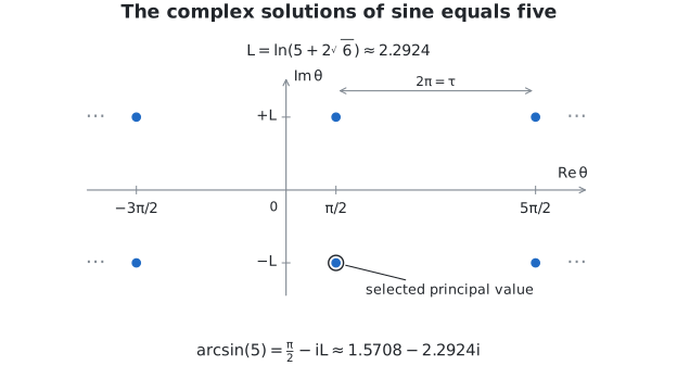
In fact, this extension works for all real numbers!
Using similar techniques, this extension can work for all of the complex numbers!
Complex Definitions of Inverse Trigonometric Functions
These inverse trigonometric functions can be extended to complex inputs by similar techniques, with exceptions: tangent and cotangent never take the values \(\pm i\), and secant and cosecant never take the value \(0\). We will focus on arcsine and arccosine, whose inverse relations exist for every complex input.
To take the arcsine of a complex number, we will use the same method as above, but with a complex input. We seek every \(\theta\) satisfying \(\sin(\theta) = z\), where \(z\) is any complex number.
Now we can expand out the sine using our complex definition,
\[\frac{e^{i\theta} - e^{- i\theta}}{2i} = z\]
Now we multiply by \(2i\) to clear the fraction:
\[e^{i\theta} - e^{- i\theta} = 2iz\]
Then we multiply by \(e^{i\theta}\), giving
\[\left( e^{i\theta} \right)^{2} - 1 = 2ize^{i\theta}\]
After rearranging the equation \(\left( e^{i\theta} \right)^{2} - 2ize^{i\theta} = 1\), we can complete the square. To complete the square, we add \({(iz)}^{2}\) to both sides, which is really just \(- z^{2}\) by the properties of \(i\).
\[\left( \left( e^{i\theta} \right) \right)^{2} - 2ize^{i\theta} - z^{2} = 1 - z^{2}\]
We collapse this into a perfect square, so
\[\left( e^{i\theta} - iz \right)^{2} = 1 - z^{2}\]
Taking square roots, we can isolate \(e^{i\theta}\)
\[e^{i\theta} - iz = \pm \sqrt{1 - z^{2}}\]
Therefore
\[e^{i\theta} = iz \pm \sqrt{1 - z^{2}}\]
Both logarithm arguments are nonzero: their product is −1. Using the Chapter 8 principal Log and its complete family gives
\[i\theta = \text{Log}\left( iz \pm \sqrt{1 - z^{2}} \right) + 2\pi ik\]
Hence
\[\theta = - i*\text{Log}\left( iz \pm \sqrt{1 - z^{2}} \right) + 2\pi k\]
This gives every inverse sine value for any complex \(z\), with either radical sign and any integer \(k\). To select one principal value, we use
\[\boxed{\arcsin(z) = - i*\text{Log}\left( iz + \sqrt{1 - z^{2}} \right)}\]
Here \(\sqrt{u} = \exp\left( \frac{\text{Log}(u)}{2} \right)\) for \(u \neq 0\), and \(\sqrt{0} = 0\), using \(- \pi < \text{Arg}(u) \leq \pi\).
This branch is analytic off the real cuts \(x \leq - 1\) and \(x \geq 1\); on the cuts, the displayed formula specifies the boundary values, including the value at 5 selected above. At \(z = \pm 1\) the two radical signs coincide, so they repeat the same family.
This formula looks very similar to the inverse sinh formula
\[{arsinh}(z) = \text{Log}\left( z + \sqrt{z^{2} + 1} \right)\]
Here we use the same principal square root and Log, so arsinh is one selected value; all solutions of
\(\sinh(v) = z\) are \(v = \text{Log}\left( z \pm \sqrt{z^{2} + 1} \right) + 2\pi ik\), for integer \(k\).
The principal branch is analytic off the imaginary cuts \(z = iy\) with \(|y| \geq 1\), and the displayed formula supplies its boundary values. In fact, there also exists an equivalence identity similar to the connection between sine and hyperbolic sine. By plugging in \(z = iw\) into our arsinh formula, we find:
\[{arsinh}(iw) = \text{Log}\left( iw + \sqrt{\left( (iw) \right)^{2} + 1} \right) = \text{Log}\left( iw + \sqrt{1 - w^{2}} \right)\]
Multiplying both sides by -i, we get
\[- i{arsinh}(iw) = - i\ \text{Log}\left( iw + \sqrt{1 - w^{2}} \right)\]
This is exactly our selected formula for arcsine!
With the same square root and Log choices on both sides, including the stated boundary values,
\[\boxed{- i\ arsinh(iw) = arcsin(w)}\]
Using similar methods, we can derive a formula for arccosine:
\(\theta = - i\text{Log}\left( z \pm i\sqrt{1 - z^{2}} \right) + 2\pi k\)
These are all solutions of \(\cos(\theta) = z\), for integer \(k\); the two logarithm arguments have product 1 and are never zero. Our selected principal value is
\[\boxed{\arccos(z) = \frac{\pi}{2} - \arcsin(z)}\]
with the boundary convention above.
For the inverse hyperbolic connection, choose any \(A\) satisfying
\[\cosh(A) = z\]
Then
\[\cos( - iA) = \cosh(A) = z\]
So \(- iA\) is an arccosine value of the same \(z\), not of \(iz\). The complete family is
\(\theta = - iA + 2\pi k\) or \(\theta = iA + 2\pi k\)
For a principal arcosh value we use
\[A = \text{Log}\left( z + \sqrt{z - 1}\sqrt{z + 1} \right)\]
Its analytic branch excludes the real cut \(x \leq 1\), and the formula fixes boundary values there. Independently selected principal arccos and arcosh values do not always satisfy \(\arccos(z) = - i{arcosh}(z)\).
Connections to the Trigonometric Cubic Formula
With our knowledge of complex trigonometric functions, we can revisit the trigonometric formulas for the cubic we had studied earlier. The algebraic cubic formula ran into trouble with three distinct real roots when we insisted on real intermediate values, but we were able to handle those cases using complex numbers. Now, we can try to extend our trigonometric and hyperbolic solutions to all cubics.
First, we need to figure out where these formulas work and where we will need complex numbers.
For real \(p\) and \(q\), the cubic
\[x^{3} + px + q = 0\]
has three distinct real roots when \(p < 0\) and \(4p^{3} + 27q^{2} < 0\).
Equivalently, its discriminant \(\Delta = - 4p^{3} - 27q^{2}\) is positive. At \(\Delta = 0\) there are repeated real roots, including the triple root 0 when \(p = q = 0\); at \(\Delta < 0\) there is one real root and a nonreal conjugate pair.
The cosine formula uses only real values when \(p < 0\) and \(\Delta \geq 0\).
The real hyperbolic methods find the lone real root when \(\Delta < 0\): sinh applies for \(p > 0\), and signed cosh for \(p < 0\). Cosh also reaches the repeated-root boundary. The case \(p = 0\) reduces directly to \(x^{3} = - q\).
The trigonometric formula to solve the depressed cubic equation is:
\[\boxed{x = 2\sqrt{- \frac{p}{3}}\cos\left( \frac{1}{3}\arccos\left( \frac{3q}{2p}\sqrt{- \frac{3}{p}} \right) - \frac{\tau k}{3} \right)}\]
Here \(\tau = 2\pi\) and \(k = 0,1,2\). For real \(p < 0\), both square roots are positive.
For any complex \(p \neq 0\), choose one value \(s\) with \(s^{2} = \frac{- p}{3}\) and use \(s\) for \(\sqrt{\frac{- p}{3}}\) and \(\frac{1}{s}\) for \(\sqrt{\frac{- 3}{p}}\); the arccosine argument is then \(u = \frac{- q}{2s^{3}}\).
Any one value \(B\) with \(\cos(B) = u\) gives the three roots as
\[\boxed{x_{k} = 2s\cos\left( \frac{B - \tau k}{3} \right)}\]
counting multiplicity. Changing \(B\) or the sign of \(s\) only permutes those roots.
When \(p = 0\) and \(q \neq 0\), use
\[x_{k} = \exp\left( \frac{\text{Log}( - q) + 2\pi ik}{3} \right)\]
when \(p = q = 0\) all three roots are 0.
The problem is, when \(p < 0\) and there is only one real root, the expression inside the arccosine is outside its domain for real-valued outputs.
For example, in the cubic \(x^{3} - 2x + 3 = 0\), the expression becomes
\[\arccos\left( \frac{3(3)}{2( - 2)}\sqrt{\frac{- (3)}{- 2}} \right) \approx \arccos( - 2.7557)\]
However, we can use our new formulas for arccosines of any number (real or complex). Choose a value \(A\) with \(\cosh(A) = u\), where \(u\) is the arccosine argument above.
Then \(- iA\) is a matching arccosine value, so we can substitute it:
\[x_{k} = 2s\cos\left( \frac{- iA}{3} - \frac{\tau k}{3} \right)\]
Now we use the familiar identity \(\cos(iz) = \cosh(z)\) to rewrite the cosine in terms of hyperbolic cosine:
\[\boxed{x_{k} = 2s\cosh\left( \frac{A}{3} - \frac{i\tau k}{3} \right)}\]
The shift becomes imaginary when we move from cosine to cosh.
In our example
\(s = \sqrt{\frac{2}{3}}\), \(u = - \left( \frac{9}{4} \right)\sqrt{\frac{3}{2}}\)
and we can take
\(A = \ln\left( c + \sqrt{c^{2} - 1} \right) + i\pi\), with \(c = - u > 1\). For \(k = 0,1,2\)
This gives approximately \(0.9466 + 0.8297i\), \(0.9466 - 0.8297i\), and \(- 1.8933\).
Substitution into \(x^{3} - 2x + 3\) gives zero (with rounding) for all three.
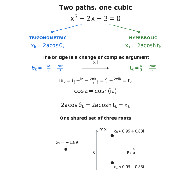
This has shown that the trigonometric and hyperbolic solutions to the cubic are really two aspects of the same formula!
Complex numbers allow for fuller descriptions of trigonometric/hyperbolic functions and their relations. This therefore allows for complex numbers to adequately describe all the solutions to the cubic without being stopped by square roots of negative numbers or the real-input restriction on arccosine, provided we keep the branch choices paired.
This relation demonstrates one of my favorite things about mathematics. We started with cubic equations from algebra, then found an unorthodox way to solve them using trigonometric identities. Later, hyperbolic functions offered another route. These seemed like completely different methods, but now we can finally see what was really going on.
The trigonometric formula did not suddenly stop working when the cubic had only one real root. The arccosine just wandered outside the real numbers! Complex numbers let us make sense of things that seemed undefined in the real numbers, like the square roots of negatives and arccosines of values outside the interval from −1 to 1.
Once we allow complex values, any cubic equation is solvable, with three roots. And the identity connecting cosine and hyperbolic cosine shows that the trigonometric and hyperbolic solutions are amazingly just two aspects of the same formula.
With these barriers broken, algebra, trigonometry, and hyperbolic trigonometry are not isolated subjects sitting in separate boxes. Through complex numbers, these three exquisite branches of mathematics turn out to be different expressions of the same ideas.
That is the beauty of mathematics.