Chapter 3: Solving Quartic Equations

Now that we know how to solve the cubic equation, let us explore the quartic equation. It is a bit more difficult than the cubic, but its solution uses many of the same concepts, such as completing the square, depressing the quartic and solving the cubic. However, there are not many visuals for these methods, so there will be more symbols without geometric interpretations. I will present two different ways of solving the quartic equation: Ferrari’s original method and an alternative method discovered by René Descartes and published in 1637.¹

Simpler Cases

Before we dive into the long process of solving the general quartic equation, it is worthwhile to discuss simpler types of quartic equations that can be solved by easier and faster methods. While not all quartics can be solved by these approaches, these approaches can save large amounts of time compared to the methods of Ferrari or Descartes if you are able to recognize these forms.

Immediately Obvious Roots

Sometimes, just by looking at the quartic equation, you can discern one or more solutions to the problem. Perhaps the simplest case is where the quartic does not contain a constant term, such as \(x^{4} + 3x^{3} - 2x^{2} + 10x = 0\).

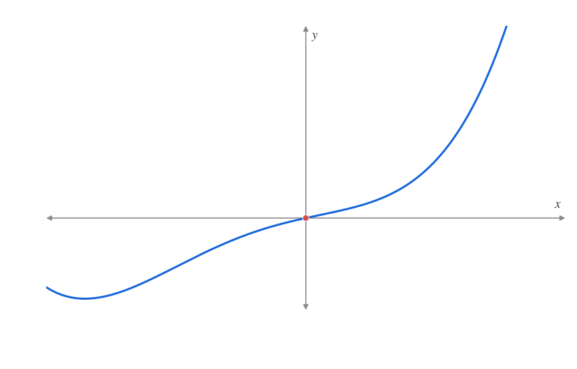
In these cases, \(x = 0\) is always a solution, and to find the remaining roots, you factor out an \(x\) and solve the remaining cubic equation by methods presented in Chapter 2. In this case, this would produce the factorization \(x\left( x^{3} + 3x^{2} - 2x + 10 \right) = 0\) and the cubic equation \(x^{3} + 3x^{2} - 2x + 10 = 0\), which can be solved to recover the remaining roots. Because all equations of this form have zero as a root, they all pass through the origin on their graphs.

Figure 3.1

If all the coefficients sum to 0, then one of the solutions is \(x = 1\). Because 1 raised to any power is still 1, all the terms cancel out. One such equation is \(x^{4} + 5x^{3} - 11x^{2} + 3x + 2 = 0\), as we can easily verify that \(1 + 5 - 11 + 3 + 2 = 0\). In this case, we can divide out the factor \((x - 1)\) from the equation using synthetic division

Figure 3.2

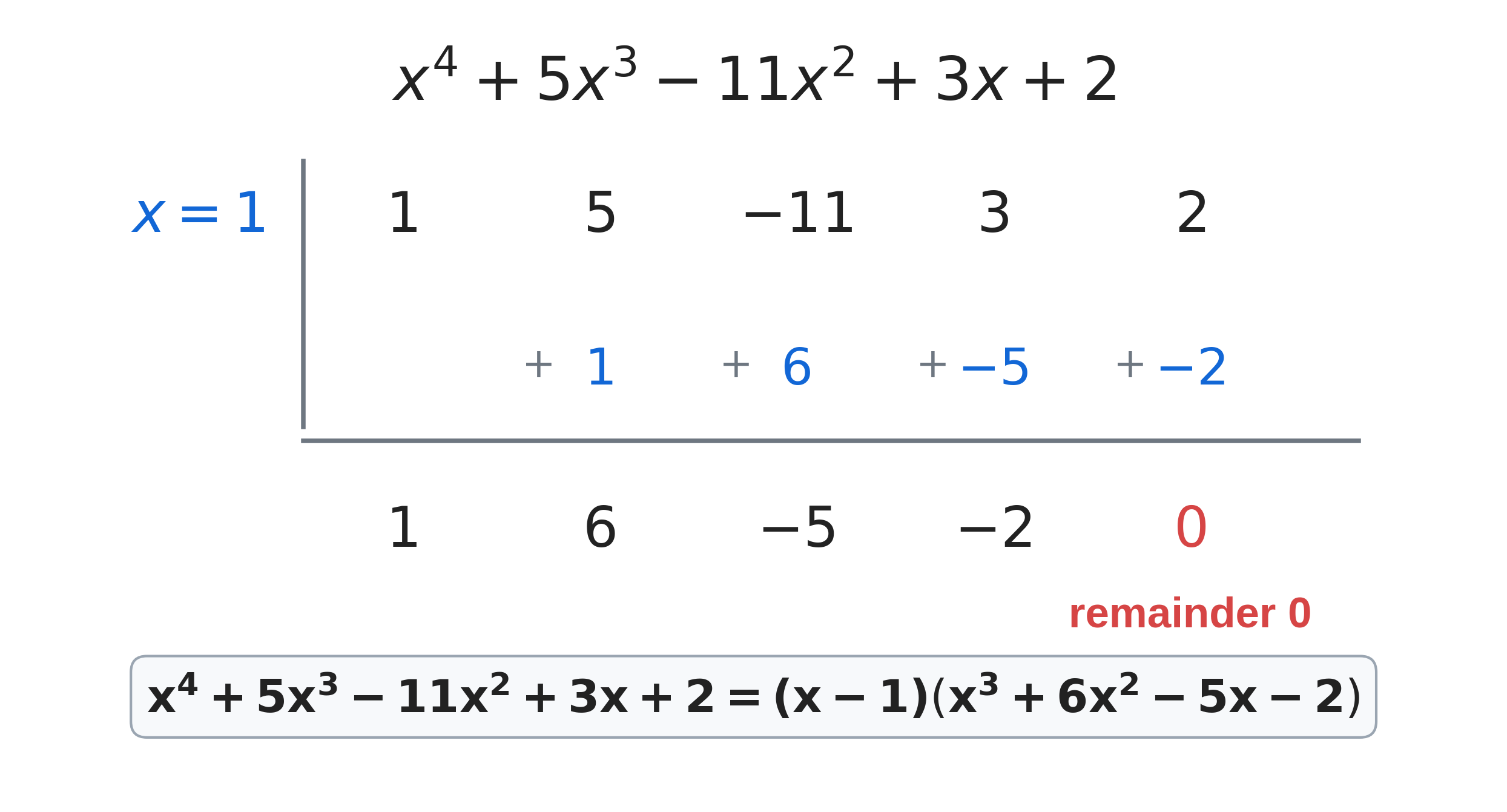
to produce a cubic equation in the remaining roots.

Similarly, if the sums of the coefficients of the even-power terms (\(x^{4},\ x^{2}\) and the constant) and the odd-power terms (\(x^{3}\) and \(x\)) are equal, then \(x = - 1\) is a solution.

This is because -1 raised to an even power becomes 1, and when raised to an odd power stays at -1. Therefore, the sum of the even terms stays the same, while the odd terms add to the negative of the sum, setting the entire expression to 0.

An example of such an equation would be \(3x^{4} + 5x^{3} + 8x^{2} + 10x + 4 = 0\). The sums of the coefficients of the even and odd terms are both 15. Therefore, \(x = - 1\) is one of the solutions to the equation. As before, we can factor out the expression \((x + 1)\) in the usual way, using synthetic division:

Figure 3.3

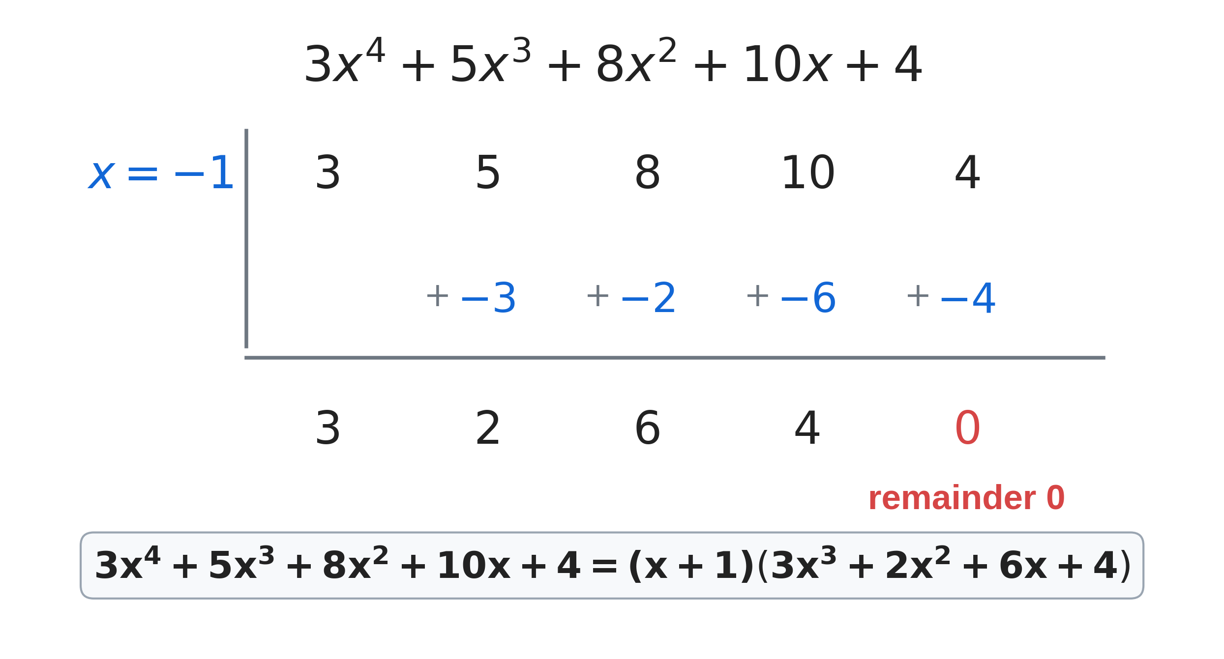
As before, this provides a cubic which, when solved, will give the other solutions to the quartic.

Biquadratic Equations

Another very special case of the quartic is known as a biquadratic equation, and it is of the form \(ax^{4} + bx^{2} + c = 0\). This type of equation is like the “disguised quadratics” we encountered in the previous chapter and has a similar method of solving.

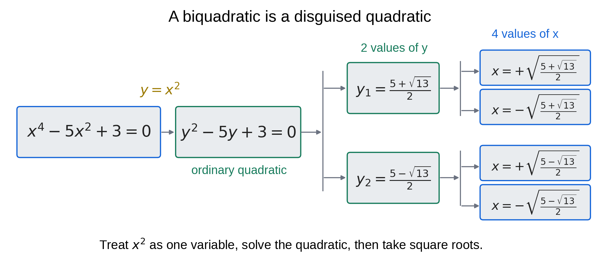
If we rewrite \(x^{4}\) as \(\left( x^{2} \right)^{2}\), this is just a quadratic equation in the variable \(x^{2}\). The name “biquadratic” translates literally as “double quadratic equation,” from how the variable in the quadratic is raised to the power of 2.

For example, the biquadratic equation \(x^{4} - 5x^{2} + 3 = 0\) can be rewritten as

\[\left( x^{2} \right)^{2} - 5x^{2} + 3 = 0\]

Then, we can solve for \(x^{2}\) using the standard quadratic formula, where \(a = 1\), \(b = - 5\) and \(c = 3\). Therefore,

\[x^{2} = \frac{5 \pm \sqrt{13}}{2}\]

Notice how there are two possibilities for the value of \(x^{2}\). Further, when we take the square root, there is another \(\pm\) sign in the solution for \(x\), so the total number of solutions for \(x\) is four. In this specific example, all four solutions for \(x\) are

\[x = \pm \sqrt{\frac{5 \pm \sqrt{13}}{2}}\]

Figure 3.4

Note: In some texts, the term “biquadratic equation” is used to refer to all quartic equations, not just this special case. In this book, the term “biquadratic equation” will only refer to this special case of equations.

Factorable Equations

All quartics, when written out in factored form, look like

\[a\left( x - x_{1} \right)\left( x - x_{2} \right)\left( x - x_{3} \right)\left( x - x_{4} \right) = 0\]

This can be rewritten as the product of two quadratic expressions if we multiply some of the factors together.

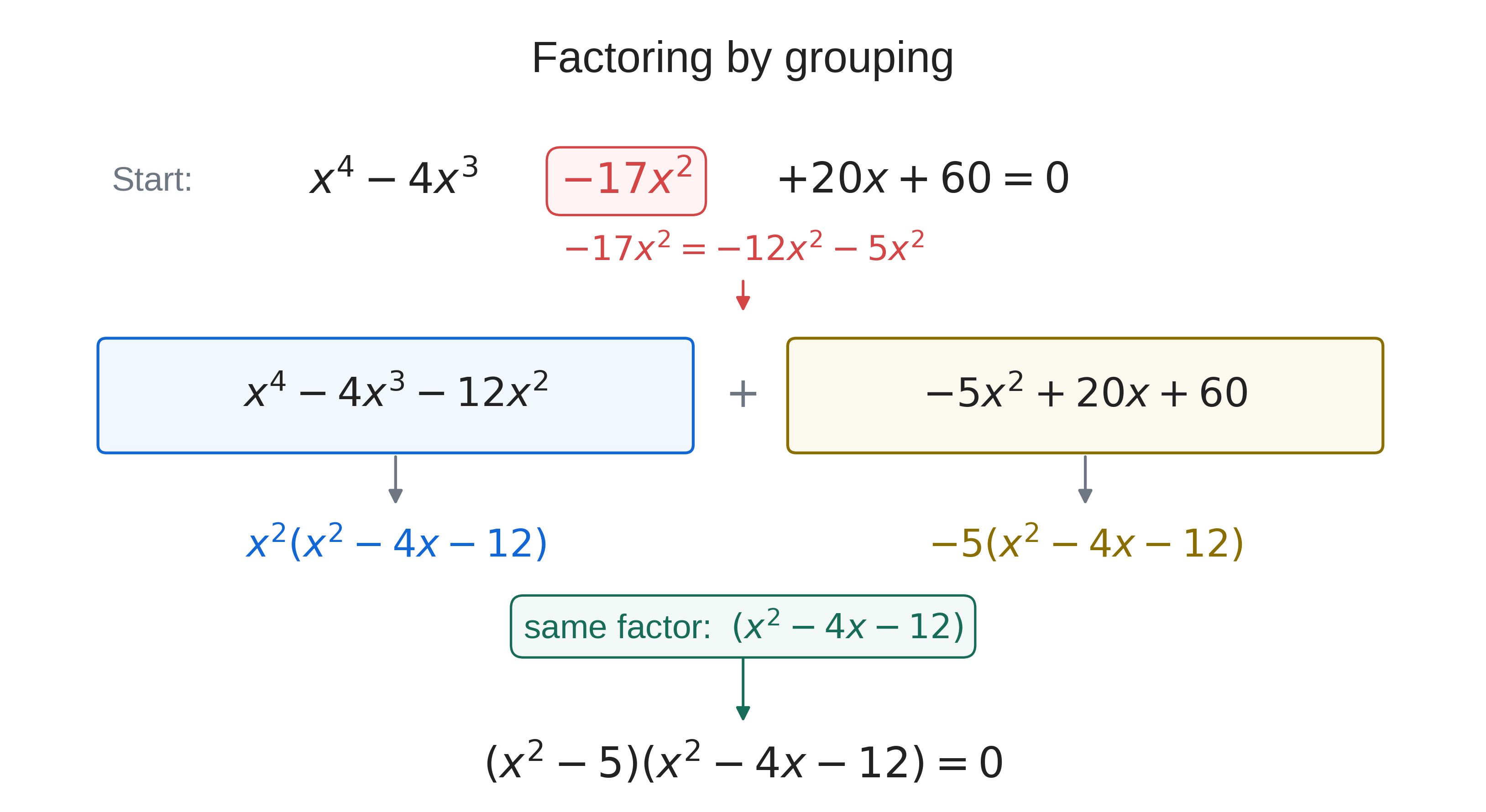
Some quartics can be nicely factored into two quadratic expressions multiplied together. This can often be done in a similar way to the factoring by grouping method in the last chapter, except that we must “split up” the \(x^{2}\) term first. As a demonstration, we are solving the equation

\[x^{4} - 4x^{3} - 17x^{2} + 20x + 60 = 0\]

While this looks difficult to solve, we can realize that \(- 17x^{2}\) can be written as \(- 12x^{2} - 5x^{2}\). This leaves

\[x^{4} - 4x^{3} - 12x^{2}\ |\ - 5x^{2} + 20x + 60\]

Then, we can focus on each half separately and see if the factors match up. In the first half, we can factor out an \(x^{2}\), leaving

\[x^{2}\left( x^{2} - 4x - 12 \right)\]

While the quadratic term is factorable into two linear terms, it is easier for this step to leave it as is. In the second half, we can factor out a -5 from each term, leaving the expression \(- 5\left( x^{2} - 4x - 12 \right)\). Now that the quadratic terms match up, we can combine the terms, forming the product

\[\left( x^{2} - 4x - 12 \right)\left( x^{2} - 5 \right) = 0\]

We can factor the first term by finding two numbers that add to -4 and multiply to -12. -6 and 2 are the correct numbers, so it factors further as

\[(x - 6)(x + 2)\left( x^{2} - 5 \right) = 0\]

The second term can be rearranged as \(x^{2} = 5\) and solved easily by taking a square root: \(x = \pm \sqrt{5}\). All four solutions are thus

\(x_{1} = 6\), \(x_{2} = - 2\), \(x_{3,4} = \pm \sqrt{5}\).

Figure 3.5

There is an easy and fast way to check if this method will work on a specific equation. First divide by the leading coefficient, so the quartic is monic. If the factorization is \(\left( x^{2} + k \right)\left( x^{2} + bx + c \right) = 0\), expanding gives \(x^{4} + bx^{3} + (c + k)x^{2} + bkx + ck = 0\).

Thus, when the cubic coefficient is nonzero, \(k\) is the linear coefficient divided by the cubic coefficient. If \(k\) is also nonzero, \(c\) is the constant divided by \(k\), and \(c + k\) must match the quadratic coefficient.

If \(k = 0\), the linear and constant coefficients must both be zero, and we can factor out \(x^{2}\).

If the cubic coefficient is zero, this factorization requires the linear coefficient to be zero too, which is the biquadratic case. If this factorization works, then you can solve for the roots as previously illustrated. If not, then this particular grouping does not work for that equation.

While we have only studied the special case where one of the quadratics is missing a \(bx\) term, this is a special case of the fact that all quartics can factor as the product of two general quadratics. However, finding these two factors is much more difficult, but still possible. This observation forms the basis for Descartes’ method, which will be explored later in this chapter.

Symmetric Quartics

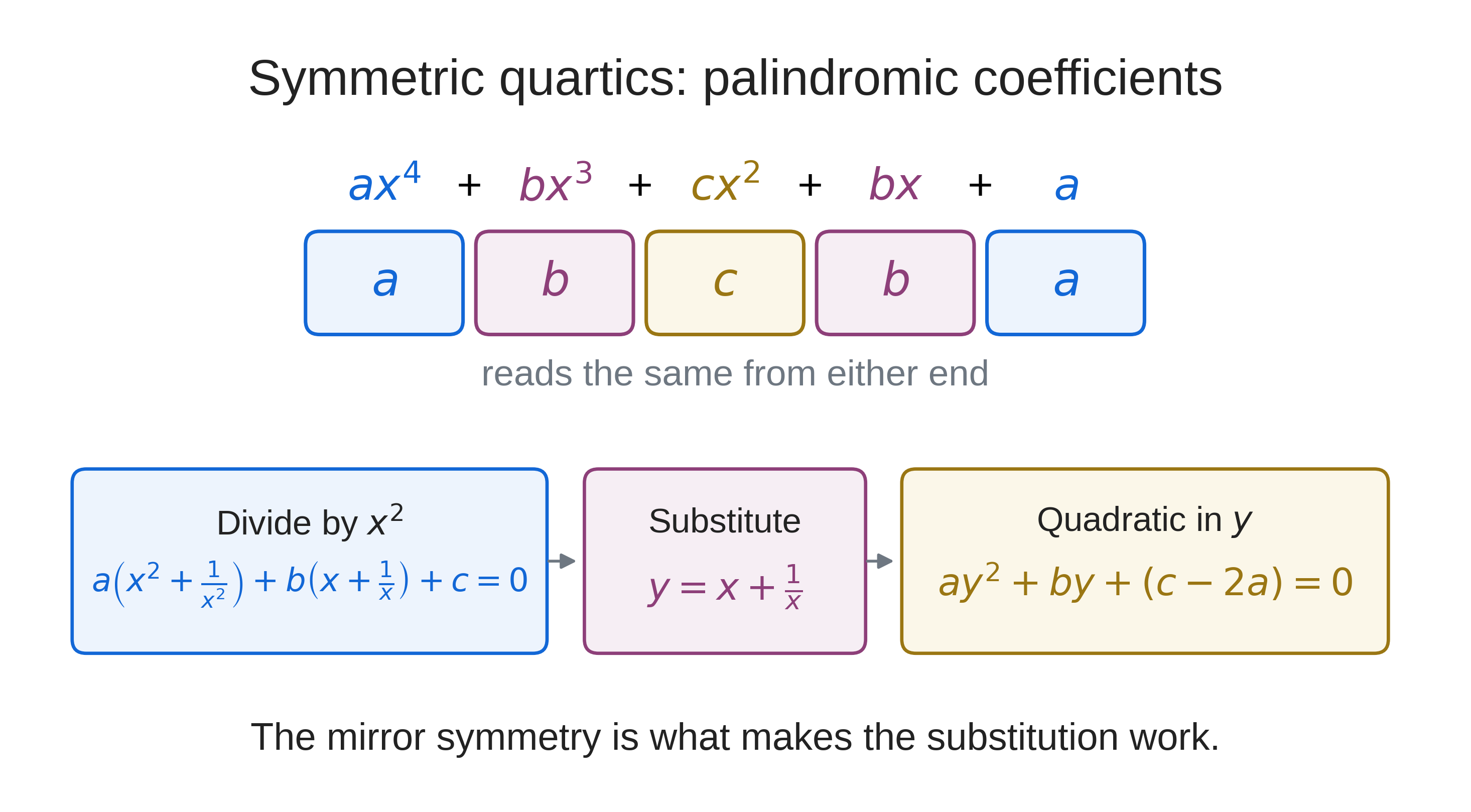
Another special case of quartics is known as symmetric equations, also called palindromic equations. They have the form \(ax^{4} + bx^{3} + cx^{2} + bx + a = 0\). The coefficients form a “palindrome,” hence the naming. This case can be solved in a very clever and special way, described here.

Figure 3.6

Since the leading coefficient \(a\) is nonzero, the constant \(a\) is also nonzero, so \(x = 0\) cannot be a root.

The first step is to divide by \(x^{2}\), forming

\[ax^{2} + bx + c + \frac{b}{x} + \frac{a}{x^{2}} = 0\]

Now we rearrange the terms

\[\left( ax^{2} + \frac{a}{x^{2}} \right) + \left( bx + \frac{b}{x} \right) + c = 0\]

And factor out constants:

\[a\left( x^{2} + \frac{1}{x^{2}} \right) + b\left( x + \frac{1}{x} \right) + c = 0\]

The second term in the equation has the expression \(\left( x + \frac{1}{x} \right)\), and we want the first term to be in the same variable, as we could substitute \(y = x + \frac{1}{x}\) and simplify the equation.

We can use the fact that, by expansion:

\[\left( x + \frac{1}{x} \right)^{2} = x^{2} + 2 + \frac{1}{x^{2}}\]

To get the first term into this form, we add \(2a\) to both sides:

\[a\left( x^{2} + \frac{1}{x^{2}} \right) + 2a + b\left( x + \frac{1}{x} \right) + c = 2a\]

\[a\left( x^{2} + 2 + \frac{1}{x^{2}} \right) + b\left( x + \frac{1}{x} \right) + c = 2a\]

\[a\left( x + \frac{1}{x} \right)^{2} + b\left( x + \frac{1}{x} \right) + c = 2a\]

Now we can substitute \(y = x + \frac{1}{x}\).

\[\boxed{ay^{2} + by + c = 2a}\]

This is a quadratic in \(y\), with standard form of \(ay^{2} + by + c - 2a = 0\).

This quadratic can be solved using the standard methods of completing the square or using the quadratic formula. Note that we obtain two solutions for \(y\).

\[y = \frac{- b \pm \sqrt{b^{2} - 4ac + 8a^{2}}}{2a}\]

We know that \(x + \frac{1}{x} = y\), so \(x^{2} + 1 = xy\). This is another quadratic in \(x\), which we can solve. \(y\) is already expressed in terms of \(a\), \(b\) and \(c\), so it is a known value.

Rearranging,

\[x^{2} - xy + 1 = 0\]

Now we can solve this using the quadratic formula as well:

\[\boxed{x = \frac{y \pm \sqrt{y^{2} - 4}}{2}}\]

The two plus-minus signs show how this equation can have up to four solutions, but some of the solutions can involve square roots of negative numbers.

There is a larger class of quartic equations, similar to symmetric equations, known as quasi-symmetric equations. The prefix quasi means “a variant of”, or “resembling”, so these equations are similar to symmetric equations.

Quasi-Symmetric Quartics

A quasi-symmetric equation is of the form \(ax^{4} + bx^{3} + cx^{2} + bmx + am^{2} = 0\). Notice how a symmetric equation is a quasi-symmetric equation where \(m = 1\), so all symmetric equations are quasi-symmetric.

Luckily, solving one uses most of the same techniques as solving symmetric equations.

First divide by \(x^{2}\).

\[ax^{2} + bx + c + \frac{bm}{x} + \frac{am^{2}}{x^{2}} = 0\]

Then, we rearrange the terms, to get like factors together:

\[ax^{2} + \frac{am^{2}}{x^{2}} + bx + \frac{bm}{x} + c = 0\]

Now we factor out \(a\) and \(b\) from the groups of terms:

\[a\left( x^{2} + \frac{m^{2}}{x^{2}} \right) + b\left( x + \frac{m}{x} \right) + c = 0\]

Again, we can write

\[\left( x + \frac{m}{x} \right)^{2} = x^{2} + 2m + \frac{m^{2}}{x^{2}}\]

Therefore,

\[x^{2} + \frac{m^{2}}{x^{2}} = \left( x + \frac{m}{x} \right)^{2} - 2m\]

By substitution, we can write:

\[a\left( \left( x + \frac{m}{x} \right)^{2} - 2m \right) + b\left( x + \frac{m}{x} \right) + c = 0\]

Now, we can substitute in a new variable to simplify:

\[y = x + \frac{m}{x}\]

\(a\left( y^{2} - 2m \right) + by + c = 0\)

This is a quadratic in \(y\), and we can solve by grouping like terms together:

\[\boxed{ay^{2} + by + c - 2ma = 0}\]

And applying the quadratic formula:

\[y = \frac{- b \pm \sqrt{b^{2} - 4ac + 8ma^{2}}}{2a}\]

Now that we know \(y\), we can isolate \(x\) from the equation

\[y = x + \frac{m}{x}\]

After multiplying through by \(x\):

\[yx = x^{2} + m\]

We bring all terms to one side:

\[x^{2} - yx + m = 0\]

Now we apply the quadratic formula again:

\[\boxed{x = \frac{y \pm \sqrt{y^{2} - 4m}}{2}}\]

Now we have our general formula for \(x\) in a quasi-symmetric equation.

Depressing the Quartic

In Ferrari’s and Descartes’ methods, it is necessary to first depress the quartic equation. We use a similar method to the cubic, but this time we substitute \(x = w - \frac{b}{4a}\).

I will use “algebra autopilot” again, as this part gets even more messy.

Figure 3.7

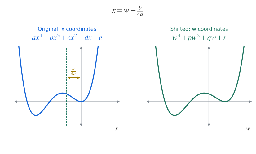
We start with the general quartic equation:

\[ax^{4} + bx^{3} + cx^{2} + dx + e = 0\]

We can divide by \(a\) to get a leading coefficient of one, so now we have:

\[x^{4} + \frac{b}{a}x^{3} + \frac{c}{a}x^{2} + \frac{d}{a}x + \frac{e}{a} = 0\]

Now we make our substitution to get rid of the cubic term:

\[\left( w - \frac{b}{4a} \right)^{4} + \frac{b}{a}\left( w - \frac{b}{4a} \right)^{3} + \frac{c}{a}\left( w - \frac{b}{4a} \right)^{2} + \frac{d}{a}\left( w - \frac{b}{4a} \right) + \frac{e}{a} = 0\]

Expanding the terms, we get:

\[\begin{aligned} &w^{4} - \frac{b}{a}w^{3} + \frac{3b^{2}}{8a^{2}}w^{2} - \frac{b^{3}}{16a^{3}}w + \frac{b^{4}}{256a^{4}} \\[1.0em] &\quad + \frac{b}{a}\left( w^{3} - \frac{3b}{4a}w^{2} + \frac{3b^{2}}{16a^{2}}w - \frac{b^{3}}{64a^{3}} \right) \\[1.0em] &\quad + \frac{c}{a}\left( w^{2} - \frac{b}{2a}w + \frac{b^{2}}{16a^{2}} \right) + \frac{d}{a}\left( w - \frac{b}{4a} \right) + \frac{e}{a} = 0 \end{aligned}\]

Distributing inside the parentheses, we obtain:

\[\begin{aligned} &w^{4} - \frac{b}{a}w^{3} + \frac{3b^{2}}{8a^{2}}w^{2} - \frac{b^{3}}{16a^{3}}w + \frac{b^{4}}{256a^{4}} \\[1.0em] &\quad + \frac{b}{a}w^{3} - \frac{3b^{2}}{4a^{2}}w^{2} + \frac{3b^{3}}{16a^{3}}w - \frac{b^{4}}{64a^{4}} \\[1.0em] &\quad + \frac{c}{a}w^{2} - \frac{bc}{2a^{2}}w + \frac{b^{2}c}{16a^{3}} + \frac{d}{a}w - \frac{bd}{4a^{2}} + \frac{e}{a} = 0 \end{aligned}\]

Now we can combine all the like terms to get the equation:

\[w^{4} + \left( - \frac{3b^{2}}{8a^{2}} + \frac{c}{a} \right)w^{2} + \left( \frac{b^{3}}{8a^{3}} - \frac{bc}{2a^{2}} + \frac{d}{a} \right)w + \left( \frac{- 3b^{4}}{256a^{4}} + \frac{b^{2}c}{16a^{3}} - \frac{bd}{4a^{2}} + \frac{e}{a} \right) = 0\]

Now we have a new quartic equation without a cubic term. I will set up new coefficients as usual to simplify things:

\[p = - \frac{3b^{2}}{8a^{2}} + \frac{c}{a}\]

\[q = \frac{b^{3}}{8a^{3}} - \frac{bc}{2a^{2}} + \frac{d}{a}\]

\[r = \frac{- 3b^{4}}{256a^{4}} + \frac{b^{2}c}{16a^{3}} - \frac{bd}{4a^{2}} + \frac{e}{a}\]

Ferrari’s Method

Factoring Into a Perfect Square

The equation \(w^{4} + pw^{2} + qw + r = 0\) is very difficult to solve, but the genius Ferrari figured out a magical way to solve it.

Figure 3.8

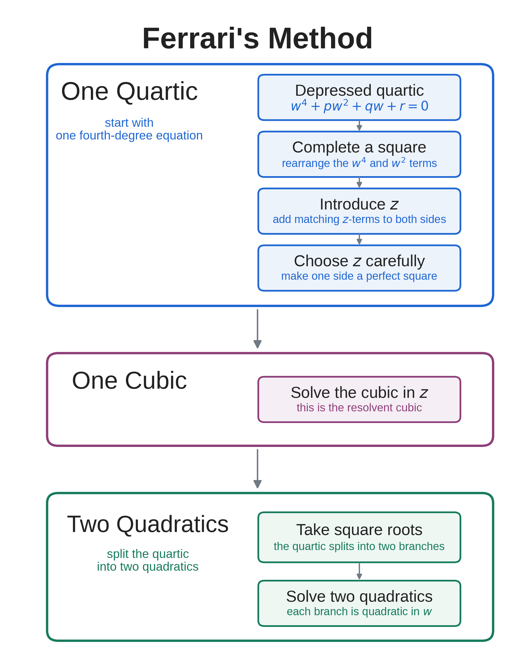
First, we can move the linear and constant terms to the right, \(w^{4} + pw^{2} = - qw - r\).

We can complete the square, treating \(w^{4}\) as our quadratic term and \(w^{2}\) as our linear term. Now we add \(pw^{2} + p^{2}\) to both sides:

\[w^{4} + 2pw^{2} + p^{2} = pw^{2} - qw + p^{2} - r\]

The left side is now a perfect square in terms of \(w^{2}\), so we can factor it as

\[{(w^{2} + p)}^{2} = pw^{2} - qw + p^{2} - r\]

Inserting the Variable z

At this stage, Ferrari proceeds to add in a new unknown term, z. The idea is to first introduce \(z\) and later set it to a specific value so the equation simplifies into something we do know how to solve.

Because \({(w^{2} + p)}^{2}\) is itself a square term, we can complete the square again in terms of \(z\). To do this, we treat \(\left( w^{2} + p \right)^{2}\) as the starting square to add on to.
We have the equation

\[\left( w^{2} + p \right)^{2} = pw^{2} - qw + p^{2} - r\]

Now we can add \(2\left( w^{2} + p \right)z + z^{2}\) to both sides to complete the square.

\[\left( w^{2} + p \right)^{2} + 2\left( w^{2} + p \right)z + z^{2} = pw^{2} - qw + p^{2} - r + 2\left( w^{2} + p \right)z + z^{2}\]

Now we complete the square as usual, giving us

\[{(w^{2} + p + z)}^{2} = pw^{2} - qw + p^{2} - r + 2\left( w^{2} + p \right)z + z^{2}\]

Combining like terms, we end up with our new equation

\[{(w^{2} + p + z)}^{2} = (p + 2z)w^{2} - qw + p^{2} + 2pz + z^{2} - r\]

Factoring the Right Side Into a Perfect Square

The left side has been folded into a perfect square, and if the right side is a perfect square, we could take square roots and solve the equation.

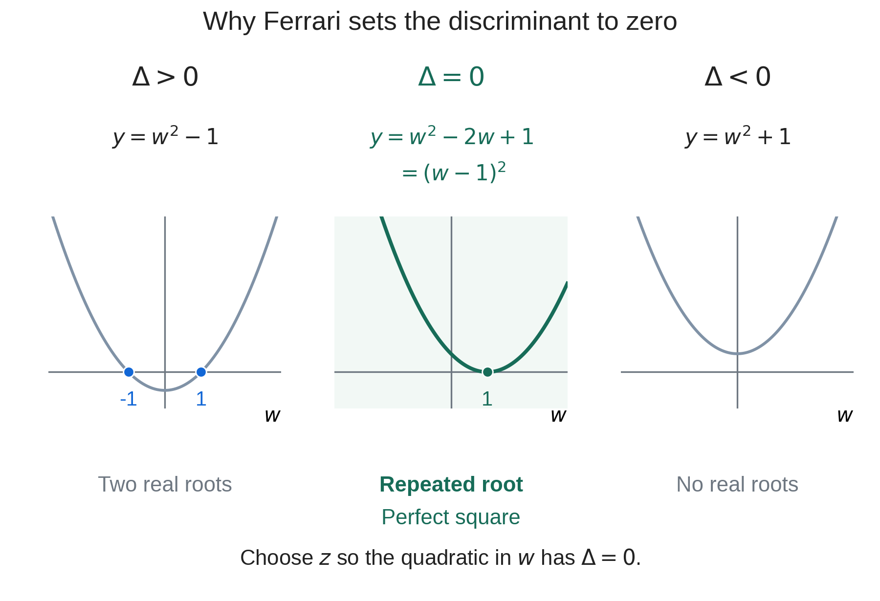
Now the goal is to specifically choose \(z\) to make the right side a perfect square. The right side is a quadratic expression, so for it to factor as a perfect square, the discriminant must be equal to zero, as mentioned in Chapter 1. Setting the discriminant equal to zero gives the equation

\[q^{2} - 4(p + 2z)\left( p^{2} + 2pz + z^{2} - r \right) = 0\]

If we can solve this equation for \(z\) in terms of \(p\), \(q\) and \(r\), the right side must factor as a perfect square.

Figure 3.9

Expanding out the terms leaves us with this equation:

\[q^{2} - 4p^{3} - 8p^{2}z - 4pz^{2} + 4pr - 8p^{2}z - 16pz^{2} - 8z^{3} + 8zr = 0\]

Now, combining like terms gives

\[- 8z^{3} - 20pz^{2} + \left( - 16p^{2} + 8r \right)z + 4pr - 4p^{3} + q^{2} = 0\]

This is a cubic equation in terms of \(z\), which we already know how to solve!

As an easy preprocessing step, we can divide by \(- 8\), giving

\[\boxed{z^{3} + \frac{5}{2}pz^{2} + \left( 2p^{2} - r \right)z - \frac{1}{2}pr + \frac{1}{2}p^{3} - \frac{1}{8}q^{2} = 0}\]

Solving the Cubic

Ferrari’s method reduces the problem to a cubic. We will solve this equation with the cubic formula, because the formula is simpler to use in this case.

The two major expressions used in the cubic formula are \(\frac{b^{3}}{27} - \frac{bc}{6} + \frac{d}{2}\) and \(- \frac{b^{2}}{9} + \frac{c}{3}\) .Here \(b\), \(c\) and \(d\) denote the coefficients of this monic cubic: \(b = \frac{5p}{2}\), \(c = 2p^{2} - r\) and \(d = \frac{p^{3}}{2} - \frac{pr}{2} - \frac{q^{2}}{8}\).

Plugging into the first expression, we get

\[\frac{b^{3}}{27} - \frac{bc}{6} + \frac{d}{2} = \frac{125}{216}p^{3} - \frac{10p^{3} - 5pr}{12} - \frac{1}{4}pr + \frac{1}{4}p^{3} - \frac{1}{16}q^{2}\]

In the second expression, we obtain \[- \frac{b^{2}}{9} + \frac{c}{3} = - \frac{25}{36}p^{2} + \frac{2p^{2} - r}{3}\]

Simplifying, our expressions are

\[\frac{b^{3}}{27} - \frac{bc}{6} + \frac{d}{2} = - \frac{1}{216}p^{3} + \frac{1}{6}pr - \frac{q^{2}}{16}\]

\[- \frac{b^{2}}{9} + \frac{c}{3} = - \frac{1}{36}p^{2} - \frac{1}{3}r\]

Now we can isolate \(z\) by using these expressions in the full cubic formula.

\[\begin{aligned} z = & \sqrt[3]{\frac{1}{216}p^{3} - \frac{1}{6}pr + \frac{q^{2}}{16} + \sqrt{\left( \frac{1}{216}p^{3} - \frac{1}{6}pr + \frac{q^{2}}{16} \right)^{2} + \left( - \frac{1}{36}p^{2} - \frac{1}{3}r \right)^{3}}} \\[1.0em] &\quad + \sqrt[3]{\frac{1}{216}p^{3} - \frac{1}{6}pr + \frac{q^{2}}{16} - \sqrt{\left( \frac{1}{216}p^{3} - \frac{1}{6}pr + \frac{q^{2}}{16} \right)^{2} + \left( - \frac{1}{36}p^{2} - \frac{1}{3}r \right)^{3}}} \\[1.0em] &\quad - \frac{5}{6}p\ \end{aligned}\]

Factoring the Right Side

Now that we have \(z\) as a known value, we can factor the right side of our original equation. Recall that the right side of our equation was

\[(p + 2z)w^{2} - qw + p^{2} + 2pz + z^{2} - r\]

If a quadratic expression of the form \(aw^{2} + bw + c\) is a perfect square, it must factor as

\[a\left( w + \frac{b}{2a} \right)^{2}\]

Rewriting:

\[{(\sqrt{a})}^{2}\left( w + \frac{b}{2a} \right)^{2}\]

Now we can distribute inside the parentheses like this:

\[\left( \sqrt{a}w + \frac{b\sqrt{a}}{2a} \right)^{2}\]

We can simplify the fraction to

\[\left( \sqrt{a}w + \frac{b}{2\sqrt{a}} \right)^{2}\]

Now we can plug in our expressions for \(a\) and \(b\), giving us perfect squares on both sides:

\[{(w^{2} + p + z)}^{2} = \left( \sqrt{p + 2z}w - \frac{q}{2\sqrt{p + 2z}} \right)^{2}\]

Now we can take square roots of both sides to get a quadratic equation, but we can’t forget to include the plus/minus sign on the right side.

\[w^{2} + p + z = \pm_{d}\sqrt{p + 2z}w \mp_{d}\frac{q}{2\sqrt{p + 2z}}\]

The d labels underneath the plus-minus and minus-plus signs mark that the signs are dependent. This means that if the first sign is a plus, then the second must be a minus and vice versa, so there are only two possibilities for the right side.

Solving for w and x

Moving everything to the left side, we get the quadratic:

\[w^{2} \mp_{d}\sqrt{p + 2z}w + p + z \pm_{d}\frac{q}{2\sqrt{p + 2z}} = 0\]

Now we can solve by the quadratic formula:

\[w = \frac{\pm_{d}\sqrt{p + 2z} \pm \sqrt{p + 2z - 4p - 4z \mp_{d}\frac{2q}{\sqrt{p + 2z}}}}{2}\]

Simplifying inside the radical, our result for \(w\) is

\[w = \frac{\pm_{d}\sqrt{p + 2z} \pm \sqrt{- 3p - 2z \mp_{d}\frac{2q}{\sqrt{p + 2z}}}}{2}\]

We can now convert from \(w\) back to \(x\), since \(x = w - \frac{b}{4a}\), so therefore

\[x = - \frac{b}{4a} + \frac{\pm_{d}\sqrt{p + 2z} \pm \sqrt{- 3p - 2z \mp_{d}\frac{2q}{\sqrt{p + 2z}}}}{2}\]

The Complete Formula

Back substituting for \(p\), \(q\) and \(r\) is difficult because it would make the formula much more complex, and back substituting for \(z\) would make the formula pretty much unreadable. Because of this, I will present “the quartic formula” as three different formulas below, to improve practicality and readability.

For a quartic \(ax^{4} + bx^{3} + cx^{2} + dx + e = 0\) whose depressed form has \(q \neq 0\), the following formulas apply. If \(q = 0\), use the biquadratic method from earlier in this chapter, since the formula below can otherwise require division by zero.

\[\boxed{p = - \frac{3b^{2}}{8a^{2}} + \frac{c}{a},q = \frac{b^{3}}{8a^{3}} - \frac{bc}{2a^{2}} + \frac{d}{a},\ r = \frac{- 3b^{4}}{256a^{4}} + \frac{b^{2}c}{16a^{3}} - \frac{bd}{4a^{2}} + \frac{e}{a}}\]

\[\begin{aligned} z = & \sqrt[3]{\frac{1}{216}p^{3} - \frac{1}{6}pr + \frac{q^{2}}{16} + \sqrt{\left( \frac{1}{216}p^{3} - \frac{1}{6}pr + \frac{q^{2}}{16} \right)^{2} + \left( - \frac{1}{36}p^{2} - \frac{1}{3}r \right)^{3}}} \\ &\quad + \sqrt[3]{\frac{1}{216}p^{3} - \frac{1}{6}pr + \frac{q^{2}}{16} - \sqrt{\left( \frac{1}{216}p^{3} - \frac{1}{6}pr + \frac{q^{2}}{16} \right)^{2} + \left( - \frac{1}{36}p^{2} - \frac{1}{3}r \right)^{3}}} \\ &\quad - \frac{5}{6}p \end{aligned}\]

\[\boxed{x = \frac{- b}{4a} + \frac{\pm_{d}\sqrt{p + 2z} \pm \sqrt{- 3p - 2z \mp_{d}\frac{2q}{\sqrt{p + 2z}}}}{2}}\]

As you can see, though Ferrari’s method was monumental for its time, it would take a very long time to actually solve a quartic equation with it. This is why I will present an alternative method next.

Descartes’ Method

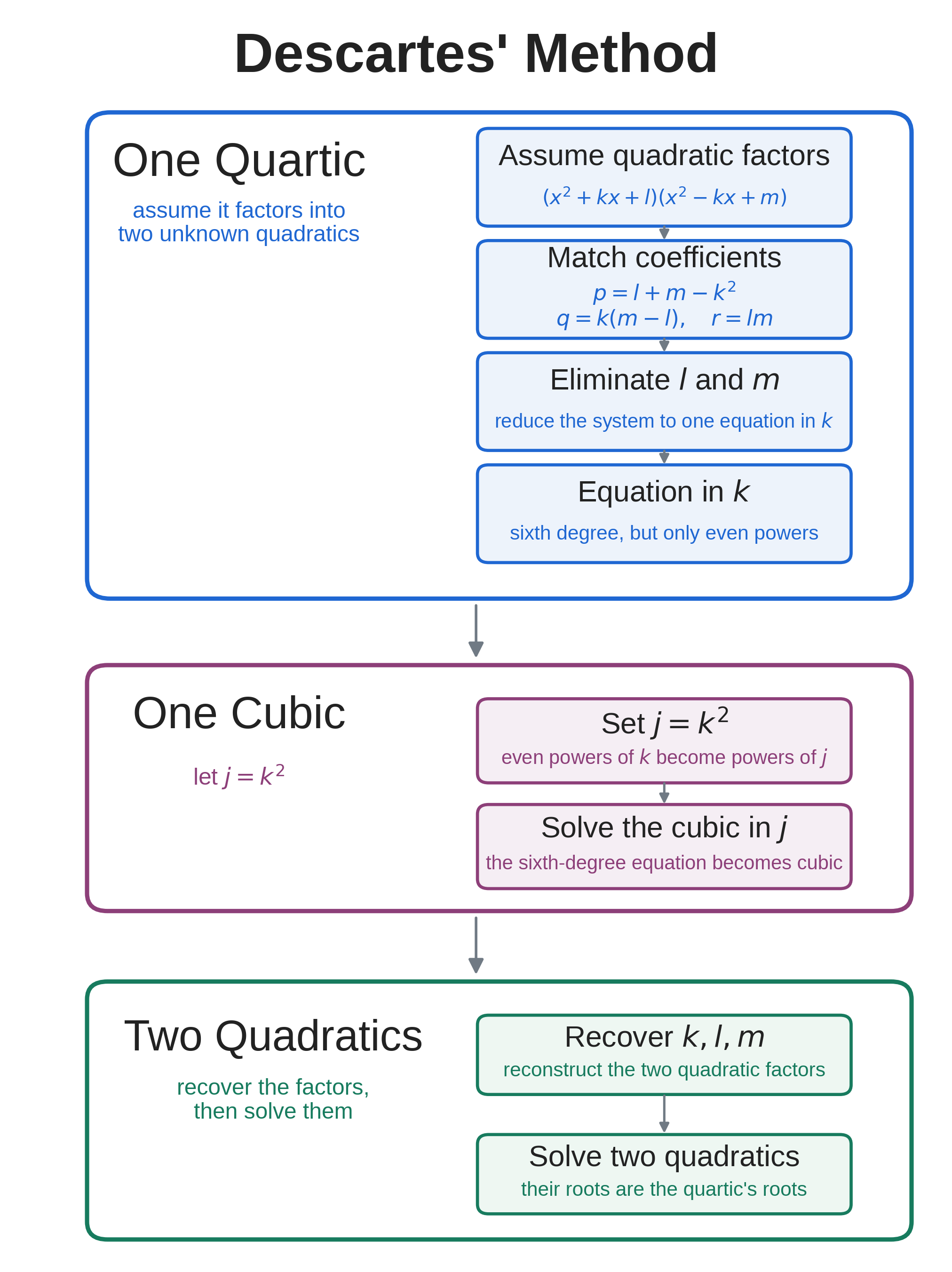
Descartes derived a method based on the fact that every quartic equation must factor into two quadratic equations.² While the coefficients of the quadratic equations are usually not rational numbers, if we can figure out what the coefficients are, then we can factor and solve from there.

Figure 3.10

Setting Up the Quadratic Factors

Here \(x\) temporarily denotes the depressed variable \(w\) from the earlier substitution. We can start with the depressed quartic equation,

\[x^{4} + px^{2} + qx + r = 0\]

and factor it into two quadratic equations with unknown coefficients:

\[\left( x^{2} + kx + l \right)\left( x^{2} + k^{'}x + m \right) = 0\]

We can now multiply out to try to find \(k\), k’, \(l\) and \(m\) in terms of \(p\), \(q\) and \(r\).

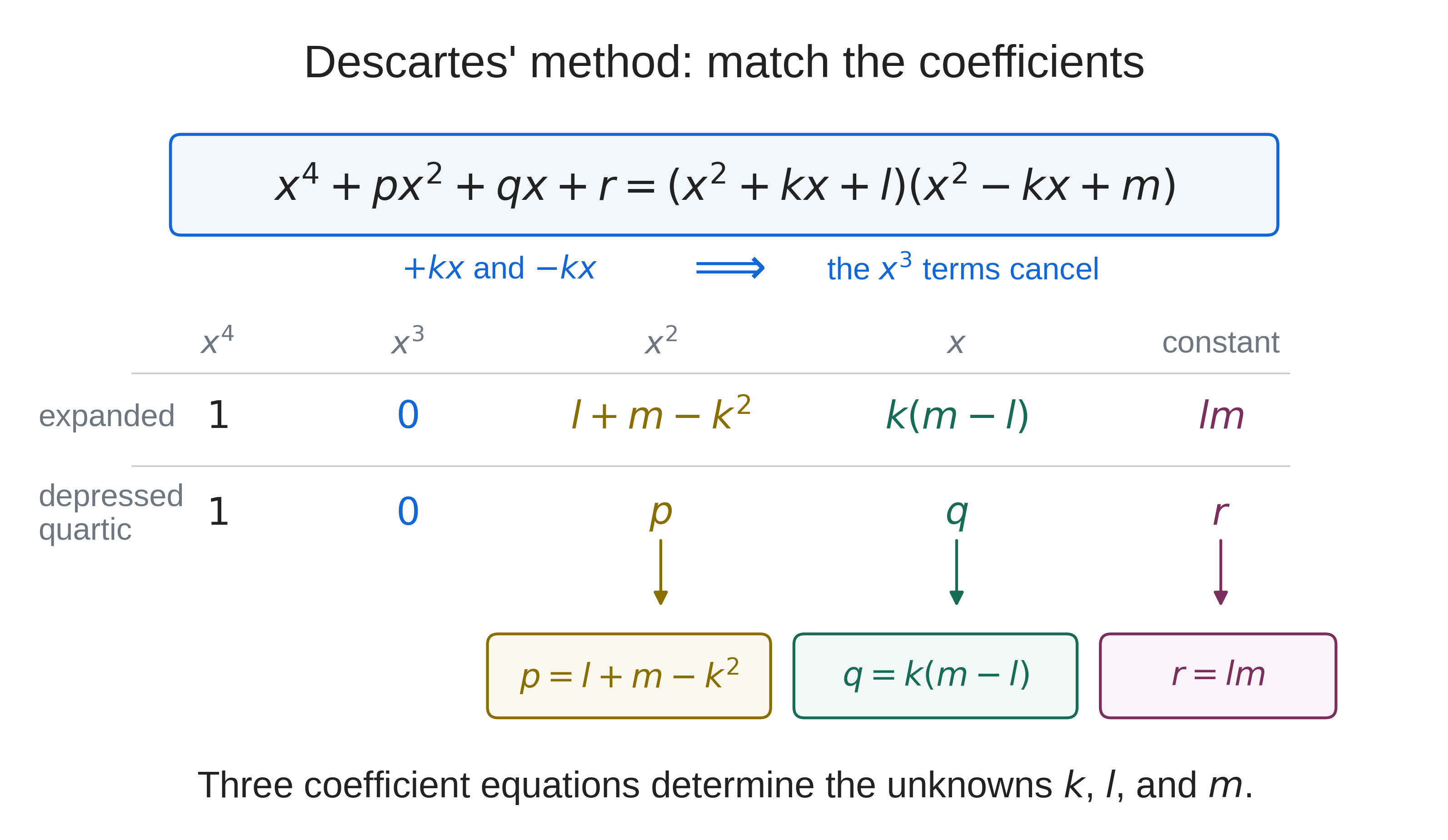
\[x^{4} + \left( k + k^{'} \right)x^{3} + \left( kk^{'} + m + l \right)x^{2} + \left( mk + lk^{'} \right)x + ml = 0\]

Because the quartic is already in depressed form, we know that \(k + k^{'} = 0\).

Therefore, \(k^{'} = - k\).

So we can substitute this in, giving

\[x^{4} + \left( - k^{2} + m + l \right)x^{2} + (mk - lk)x + ml = 0\]

Now we can match up these coefficients to our original \(p\), \(q\) and \(r\) terms, and then try to solve from there. Remember, \(p\), \(q\) and \(r\) are already known, while \(k\), \(l\), and \(m\) are unknown.

Matching our coefficients, we get a system of three equations:

\[\left\{\begin{aligned} -k^{2} + m + l &= p \\ mk - lk &= q \\ ml &= r \end{aligned}\right.\]

Figure 3.11

Solving the System

It is not immediately obvious how we could solve a system like this, but it is possible through clever substitutions.

If \(q = 0\), the depressed equation is biquadratic and can be solved by the earlier method. For the remaining case \(q \neq 0\), since \(q = k(m - l)\), \(k\) cannot be zero. We can therefore divide by \(k\) in equation 2 to obtain \(m - l = \frac{q}{k}\).

Because the first equation has the terms \(l + m\), we can eliminate \(l\) by adding the two equations like this:

\(\ - k^{2} + m + l = p\)

\(+ \ \ \ \ \ \ \ \ \ \ \ \ m - l = \frac{q}{k}\)

\(\_\_\_\_\_\_\_\_\_\_\_\_\_\_\_\_\_\_\_\_\)____

\(\ \ - k^{2} + 2m\ \ \ = p + \frac{q}{k}\)

And we can also get an equation without \(m\) by subtraction:

\(- k^{2} + m + l = p\)

\(- \ \ \ \ \ \ \ \ \ \ m - l = \frac{q}{k}\)

\(\_\_\_\_\_\_\_\_\_\_\_\_\_\_\_\_\_\_\_\_\_\_\)

\(- k^{2}\ \ \ \ \ \ \ \ + 2l = p - \frac{q}{k}\).

We can solve both of these equations for either \(m\) or \(l\), giving us two new equations:

\[2l = k^{2} + p - \frac{q}{k},\ \ \ \ \ 2m = k^{2} + p + \frac{q}{k}\]

In equation 3, we know that \(ml = r\). Therefore,

\[(2m)(2l) = 4r\]

So we can substitute our first two equations to get an equation in only \(k\) that we can solve.

\[\left( k^{2} + p - \frac{q}{k} \right)\left( k^{2} + p + \frac{q}{k} \right) = 4r\]

After expanding and cancelling, we find

\[k^{4} + 2pk^{2} + p^{2} - \frac{q^{2}}{k^{2}} = 4r\]

We now multiply through by \(k^{2}\) to find that

\[k^{6} + 2pk^{4} + p^{2}k^{2} - q^{2} = 4rk^{2}\]

Moving terms, we get a degree six equation of

\[k^{6} + 2pk^{4} + (p^{2} - 4r)k^{2} - q^{2} = 0\]

This equation looks intimidating, but if we consider \(k^{2}\) as a new variable \(j\), so \(j = k^{2}\), we are really dealing with a cubic equation

\[\boxed{j^{3} + 2pj^{2} + \left( p^{2} - 4r \right)j - q^{2} = 0}\]

We can now solve the equation for \(j\) using the cubic formula.

Solving the Cubic

We first need to find the expressions \(\frac{b^{3}}{27} - \frac{bc}{6} + \frac{d}{2}\), and \(- \frac{b^{2}}{9} + \frac{c}{3}\).

Plugging in, we get these expressions:

\[\frac{b^{3}}{27} - \frac{bc}{6} + \frac{d}{2} = - \frac{1}{27}p^{3} + \frac{4}{3}pr - \frac{q^{2}}{2}\]

\[- \frac{b^{2}}{9} + \frac{c}{3} = - \frac{1}{9}p^{2} - \frac{4}{3}r\]

Now our final solution for \(j\) is:

\[\begin{aligned} j = & \sqrt[3]{\frac{1}{27}p^{3} - \frac{4}{3}pr + \frac{q^{2}}{2} + \sqrt{\left( - \frac{1}{27}p^{3} + \frac{4}{3}pr - \frac{q^{2}}{2} \right)^{2} + \left( - \frac{1}{9}p^{2} - \frac{4}{3}r \right)^{3}}} \\[1.0em] &\quad + \sqrt[3]{\frac{1}{27}p^{3} - \frac{4}{3}pr + \frac{q^{2}}{2} - \sqrt{\left( - \frac{1}{27}p^{3} + \frac{4}{3}pr - \frac{q^{2}}{2} \right)^{2} + \left( - \frac{1}{9}p^{2} - \frac{4}{3}r \right)^{3}}} \\[1.0em] &\quad - \frac{2}{3}p \end{aligned}\]

Now we can solve for \(k\), because \(k^{2} = j\). Therefore, \(k = + \sqrt{j}\). The plus sign here selects one square root, possibly complex. Using the other sign would exchange \(l\) and \(m\) and swap the two quadratic factors, giving the same roots. So our solution for \(k\) is:

\[k = \left( \begin{aligned} &\sqrt[3]{\frac{1}{27}p^{3} - \frac{4}{3}pr + \frac{q^{2}}{2} + \sqrt{\left( - \frac{1}{27}p^{3} + \frac{4}{3}pr - \frac{q^{2}}{2} \right)^{2} + \left( - \frac{1}{9}p^{2} - \frac{4}{3}r \right)^{3}}} \\[1.0em] &\quad + \sqrt[3]{\frac{1}{27}p^{3} - \frac{4}{3}pr + \frac{q^{2}}{2} - \sqrt{\left( - \frac{1}{27}p^{3} + \frac{4}{3}pr - \frac{q^{2}}{2} \right)^{2} + \left( - \frac{1}{9}p^{2} - \frac{4}{3}r \right)^{3}}} \\[1.0em] &\quad - \frac{2}{3}p \end{aligned} \right)^{\frac{1}{2}}\]

Since we know \(k\), we can figure out \(m\) and \(l\) from the equations we derived earlier.

\[- k^{2} + 2m = p + \frac{q}{k}\]

We move everything but \(m\):

\[2m = k^{2} + p + \frac{q}{k}\]

And then divide by two, giving us an expression for \(m\):

\[m = \frac{k^{2}}{2} + \frac{p}{2} + \frac{q}{2k}\]

Repeating the same process for \(l\) gives:

\[- k^{2} + 2l = p - \frac{q}{k}\]

\[2l = k^{2} + p - \frac{q}{k}\]

\[l = \frac{k^{2}}{2} + \frac{p}{2} - \frac{q}{2k}\]

Solving Each Quadratic

Now that we know \(k\), \(l\) and \(m\) in terms of the original coefficients, we can factor our equation into:

\[\left( x^{2} + kx + l \right)\left( x^{2} - kx + m \right) = 0\]

Since these two quadratic expressions are multiplied together to get zero, we can set each equation equal to zero and solve from there:

\[\begin{gathered} x^{2} + kx + l = 0, \\ x^{2} - kx + m = 0 \end{gathered}\]

We solve each by the quadratic formula, to get our four solutions for \(x\):

\[x_{1,2} = \frac{- k \pm \sqrt{k^{2} - 4l}}{2}\]

\[x_{3,4} = \frac{k \pm \sqrt{k^{2} - 4m}}{2}\]

Again, the formulas would be too complicated to plug into a single “quartic formula”, so I will again present the solution as separate formulas.

This method solves a depressed quartic equation, but any quartic equation can be converted into this form, so this method can solve any quartic equation. The four values just found belong to the depressed variable. To return to the original variable in the formulas below, subtract \(\frac{b}{4a}\) from each value.

For the equation \(ax^{4} + bx^{3} + cx^{2} + dx + e = 0\):

\[p = - \frac{3b^{2}}{8a^{2}} + \frac{c}{a},q = \frac{b^{3}}{8a^{3}} - \frac{bc}{2a^{2}} + \frac{d}{a},\ r = \frac{- 3b^{4}}{256a^{4}} + \frac{b^{2}c}{16a^{3}} - \frac{bd}{4a^{2}} + \frac{e}{a}\]

\(k = \left( \sqrt[3]{\frac{1}{27}p^{3} - \frac{4}{3}pr + \frac{q^{2}}{2} + \sqrt{\left( - \frac{1}{27}p^{3} + \frac{4}{3}pr - \frac{q^{2}}{2} \right)^{2} + \left( - \frac{1}{9}p^{2} - \frac{4}{3}r \right)^{3}}} + \sqrt[3]{\frac{1}{27}p^{3} - \frac{4}{3}pr + \frac{q^{2}}{2} - \sqrt{\left( - \frac{1}{27}p^{3} + \frac{4}{3}pr - \frac{q^{2}}{2} \right)^{2} + \left( - \frac{1}{9}p^{2} - \frac{4}{3}r \right)^{3}}} - \frac{2}{3}p \right)^{\frac{1}{2}}\)

\[\begin{gathered} \boxed{m = \frac{k^{2}}{2} + \frac{p}{2} + \frac{q}{2k}} \\ \boxed{l = \frac{k^{2}}{2} + \frac{p}{2} - \frac{q}{2k}} \end{gathered}\]

\[\begin{gathered} \boxed{x_{1,2} = - \frac{b}{4a} + \frac{- k \pm \sqrt{k^{2} - 4l}}{2}} \\ \boxed{x_{3,4} = - \frac{b}{4a} + \frac{k \pm \sqrt{k^{2} - 4m}}{2}} \end{gathered}\]

What About the Quintic?

Now that we have successfully found methods to solve quadratic, cubic and quartic equations, you might wonder, “How do you solve the quintic equation?” To answer this question, we must travel back to the late 18th century, where recent advances in algebra had led many great mathematicians to ask this question themselves.

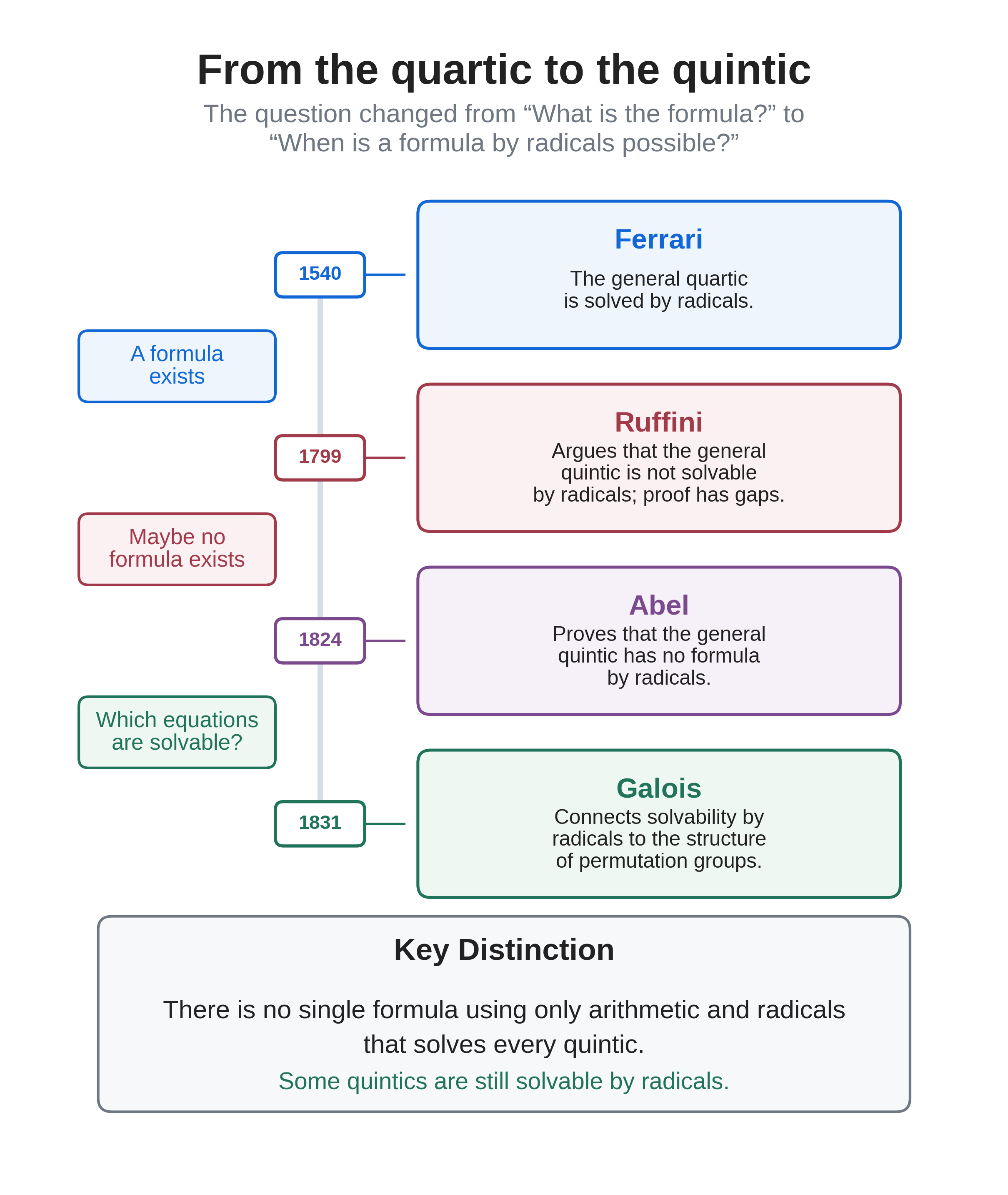
Despite the breakthroughs in Cardano’s time, no mathematician had managed to find a general radical formula for the quintic. The Italian mathematician Paolo Ruffini published an attempted proof in 1799 that no such formula exists, but it relied on an assumption that was not proven and thus was incomplete. His 1799 book ran to more than 500 pages. He sent his work to many mathematicians, but it often went unacknowledged. The great Augustin-Louis Cauchy endorsed Ruffini’s work in 1821, but the proof still had a gap.³

For the next chapter of our story, we turn to the Norwegian mathematician Niels Abel. He worked in obscurity for most of his life, and after years of work published his proof that no general radical formula exists for the quintic in 1824, in only SIX pages! He published a more complete account in 1826. This was a landmark result for the field of algebra, and Abel soon tried to find out specifically which equations could be solved by radicals, and which could not. He died in 1829 after many other significant contributions to mathematics, but never fully answered this question.⁴

For the final chapter in this story, we turn to the genius who revolutionized abstract algebra, Évariste Galois. He became absorbed in mathematics at the age of 15, and by his late teen years was already writing advanced papers. Despite his clear brilliance, he twice failed the entrance examination to École Polytechnique, one of France’s leading schools for mathematics. Later stories blamed the examiner, but the reasons for his failure are uncertain.⁵

Galois approached the problem by asking what happens when the roots of an equation are exchanged. For a polynomial with rational coefficients, some exchanges preserve all the algebraic relations among its roots with rational coefficients. Together, these permitted exchanges form what we now call its Galois group. The structure of this group tells us whether the roots can be expressed using radicals.

In modern language, an equation is solvable by radicals exactly when its Galois group is a “solvable group.” This word has a precise meaning in group theory; it is a condition on the structure of the group, not just another way of saying that we have found the roots. We will not develop that theory here, but its consequence is remarkable. It explains both why some equations of degree five or higher can be solved by radicals and why there is no radical formula that works for all of them.⁶

Galois’s work reached a wider mathematical audience when Liouville published it in 1846.⁷ The search for formulas had led to a new way of studying the relationships between roots.

Figure 3.12

But Is It Truly Unsolvable?

While I have talked at length about how the quintic is unsolvable, what does that really mean? Up through this chapter, we have been solving polynomials by radicals, which means using only basic arithmetic operations and roots. What they really proved was that it is not possible to solve all quintic equations by just those tools alone, and Galois theory can show which equations we can solve by radicals and which we can’t. It does not mean that these equations will never be solved. In fact, using more advanced tools like hyperelliptic functions and differential resolvents, which are far beyond the scope of this book, we CAN solve all quintic equations.⁸ The Abel-Ruffini theorem just sets limits on how these roots can be found and expressed.

← Previous: Chapter 2 Book contents Next: Chapter 4 →

Footnotes

1. Harald Helfgott and Michel Helfgott, “A Modern Vision of the Work of Cardano and Ferrari on Quartics,” Convergence (Mathematical Association of America, February 2010), https://doi.org/10.4169/loci003312.

2. Helfgott and Helfgott, “A Modern Vision of the Work of Cardano and Ferrari on Quartics.”

3. Luigi Pepe, “Teoria generale delle equazioni … (1799),” Matematica Italiana, Il Giardino di Archimede, https://archimede.dimai.unifi.it/archimede/matematicaitaliana/schede_opere/5ruffini99.html; Christian Houzel, “The Work of Niels Henrik Abel,” in The Legacy of Niels Henrik Abel, ed. Olav Arnfinn Laudal and Ragni Piene (Berlin: Springer, 2004), 49–52, https://abelprisen.no/sites/default/files/2021-05/houzel_the_work.pdf.

4. Houzel, “The Work of Niels Henrik Abel,” 49–52; J. J. O’Connor and E. F. Robertson, “Niels Henrik Abel,” MacTutor History of Mathematics Archive, University of St Andrews, https://mathshistory.st-andrews.ac.uk/Biographies/Abel/.

5. Tony Rothman, “Genius and Biographers: The Fictionalization of Évariste Galois,” American Mathematical Monthly 89, no. 2 (1982): 84–106, https://doi.org/10.1080/00029890.1982.11995389.

6. Évariste Galois, “Œuvres mathématiques d’Évariste Galois,” with introduction by Joseph Liouville, Journal de mathématiques pures et appliquées, 1st ser., 11 (1846): 381–444, especially 417–44, https://www.numdam.org/item/JMPA_1846_1_11\_\_381_0.pdf.

7. Galois, “Œuvres mathématiques,” 381–84.

8. Angel Zhivkov, “Resolution of Degree ≤6 Algebraic Equations by Genus Two Theta Constants,” preprint (2002), https://doi.org/10.18452/2623; Alin Bostan, Frédéric Chyzak, Grégoire Lecerf, Bruno Salvy, and Éric Schost, “Differential Equations for Algebraic Functions,” in Proceedings of ISSAC 2007 (New York: ACM, 2007), 25–32, https://arxiv.org/abs/cs/0703121.