Chapter 2: Solving Cubic Equations

Now that we have reviewed quadratic equations, we are ready to confront the cubic equation. While quadratic equations relate \(x^{2}\), \(x\) and constant terms, cubic equations add on \(x^{3}\) terms. They are not often taught in standard algebra courses due to their solutions being more complicated than those of quadratics, but they are still manageable. These equations occur in ancient unsolved problems and constants similar to the golden ratio, and they are crucial in solving quartic equations.

Historical Background

I find the history of the discovery of the cubic formula just as interesting as the methods themselves. This historical context helps explain the cubic equation.

Problems that we would now write as quadratic equations were solved around 1800 BC by the Babylonians. Related methods were developed in Persia, India and China.¹ However, a general formula for cubic equations remained out of reach. One of the most influential Persian mathematicians, Omar Khayyam, said “We have tried to find an algebraic solution to these roots, but we have failed. It may be, however, that men who come after us will succeed.” He did find a geometric solution using the conic sections of a circle and hyperbola, but was unable to provide an algebraic expression, or formula, to solve the cubic.² A general formula using radicals remained elusive for centuries, until one Italian mathematician changed everything.

The earliest known discovery of a formula using radicals for a cubic is credited to Scipione del Ferro, an Italian mathematician who lived from 1465 to 1526. He discovered a solution to a class of cubics, which we can write in modern notation in the form \(ax^{3} + bx + \, c = 0\). Lacking an \(x^{2}\) term, they are known as depressed cubic equations. These equations are a subset of cubic equations with simpler solutions. Del Ferro is not known to have given a solution for general cubic equations of the form \(ax^{3} + bx^{2} + cx + d = 0\). Nevertheless, this was a huge achievement. He was the first to discover this for literally thousands of years! But he kept it from publication, sharing it with only a few people.³

This was because, at the time, mathematicians competed for fame in mathematical “duels.” A challenge could put your reputation and prospects as a mathematician on the line. Having a secret weapon of this magnitude was a massive advantage against the competition.

Del Ferro kept his solution literally unto the grave. According to the traditional account, on his deathbed, he told his student, Antonio Fior, his solution. Fior then proceeded to brag to other mathematicians about how he had solved the cubic. He got so cocky that he challenged another well-respected mathematician, Niccolo Tartaglia, to a duel. Tartaglia had already solved problems of a different cubic type, involving a square term, given to him by a fellow mathematician.

Tartaglia sent a variety of problems to Fior, while Fior kept “all his eggs in one basket” and sent 30 depressed cubics. Tartaglia was panicking, as solving depressed cubics was difficult without del Ferro’s secret method, and there were 30 of them! In addition, he had worked for years to build his reputation, as he was self-taught without a college education. According to Tartaglia’s account, eight days before his time ran out, he independently derived a rule for the type of depressed cubic Fior had sent! He then proceeded to solve all of Fior’s problems in only two hours. Meanwhile, Fior made little headway with Tartaglia’s problems.⁴

Fior lost the duel by a long shot and dropped out of the picture. In contrast, Tartaglia became a mathematical celebrity. Mathematicians across Europe were very interested in the cubic now, especially Gerolamo Cardano, a mathematician and physician based in Milan.

Cardano was a fascinating character, a student of both medicine and math, and had a very interesting life. He wanted to know the solution to the cubic so badly that he sent letters incessantly to Tartaglia. Eventually, Tartaglia gave in when Cardano offered an introduction to a powerful patron and promised secrecy. In 1539, Tartaglia revealed the solution to the cubic as a poem, using words rather than our modern mathematical notation. According to Tartaglia’s account, Cardano swore an oath to God never to publish the solution, and to write it only in cipher.⁵

Cardano was elated by this discovery and soon began exploring other possibilities. Tartaglia did not provide him with a derivation of the method, but Cardano soon figured out the math behind the solution for himself. He then tried to extend Tartaglia’s method to discover a solution to the general cubic equation: \(ax^{3} + bx^{2} + cx + d = 0\). Amazingly, he found a process to turn any general cubic equation into a depressed cubic, which he already knew how to solve.⁶ He was so excited, he wanted to publish his result. He made his living as a physician, so he didn’t need to keep it a secret. But he had promised never to publish the solution.

Cardano proceeded to tell his student and assistant Lodovico Ferrari of his work on cubic equations. The paradigm shift came in 1540, when Ferrari discovered how to solve all quartic equations, of the form \(ax^{4} + bx^{3} + cx^{2} + dx + e = 0\) (\(e\) being a coefficient, not Euler's number). However, Ferrari’s solution involved an intermediate step of solving a cubic equation. The good news was that he knew how to solve cubics, as Cardano told him his results. The bad news was that the vow of secrecy Cardano made was still in effect, so he could not publish his results either.⁷

“Team Cardano” really wanted to publish, but they couldn’t. However, Cardano and Ferrari were undeterred. They were able to trace back the cubic solution to Scipione del Ferro, the original discoverer. They travelled to Bologna, del Ferro’s hometown, to investigate. They managed to track down Scipione’s son-in-law, and he presented Cardano with one of del Ferro’s notebooks that had been in their family for some time. The notebook contained Del Ferro’s original solution to depressed cubic equations. In Cardano’s view, this freed him from his oath. He believed he could publish del Ferro’s earlier discovery without revealing a secret that belonged to Tartaglia alone. He started writing, and in 1545 published Ars Magna, “The Great Art”.⁸

Ars Magna is often regarded as one of the works marking the beginning of modern algebra. The solution spread all over Europe, and eventually around the world. However, Tartaglia was livid at this supposed breach of oath. He sent Cardano insulting letters constantly. It escalated from there: Ferrari challenged Tartaglia to a duel, while Tartaglia wanted to face Cardano himself.

Cardano did not take part, and Ferrari faced Tartaglia. This time, the duel was public in the middle of Milan, so the stakes were even higher. Ferrari is generally regarded as winning the first day, and Tartaglia gave up and left town before continuing. His reputation suffered, but he continued writing mathematics.⁹

Ars Magna won Cardano and Ferrari everlasting fame. In fact, the modern interpretation of Tartaglia and del Ferro’s solution is often called “Cardano’s method”, even though he developed proofs and extended the method to general cubics, rather than first discovering the depressed-cubic rule. In addition, the first solution to the quartic is called Ferrari’s method.

The cubic formula had one slight problem, however. It sometimes forced you to take the square root of a negative number, which is outside of the real numbers. But the cubic could have an obvious real solution, say \(4\), that was expressed in terms of these weird negative square roots. Cardano and his contemporaries were totally freaked out by this. It is known as the “casus irreducibilis”, the irreducible case.¹⁰

Completing the Cube

Just as we can complete the square for quadratic equations, it is possible to “complete the cube” for cubic equations. This method has both a geometric interpretation in terms of shapes, and an algebraic interpretation in terms of symbols.

To demonstrate Tartaglia’s solution, I will first solve a specific depressed cubic equation and then solve it in the general case.¹¹ We will try and solve the equation:

\[x^{3} + 3x = 5\]

This equation is not factorable over the rationals and does not have rational roots. In this geometric interpretation, as with completing the square, we try to add onto the cube to make a larger cube. Adding on a distance of \(y\), which is unknown currently, forms a larger cube. We can call the total side length of the new cube, \(z\ = \ x + y\).

Figure 2.1

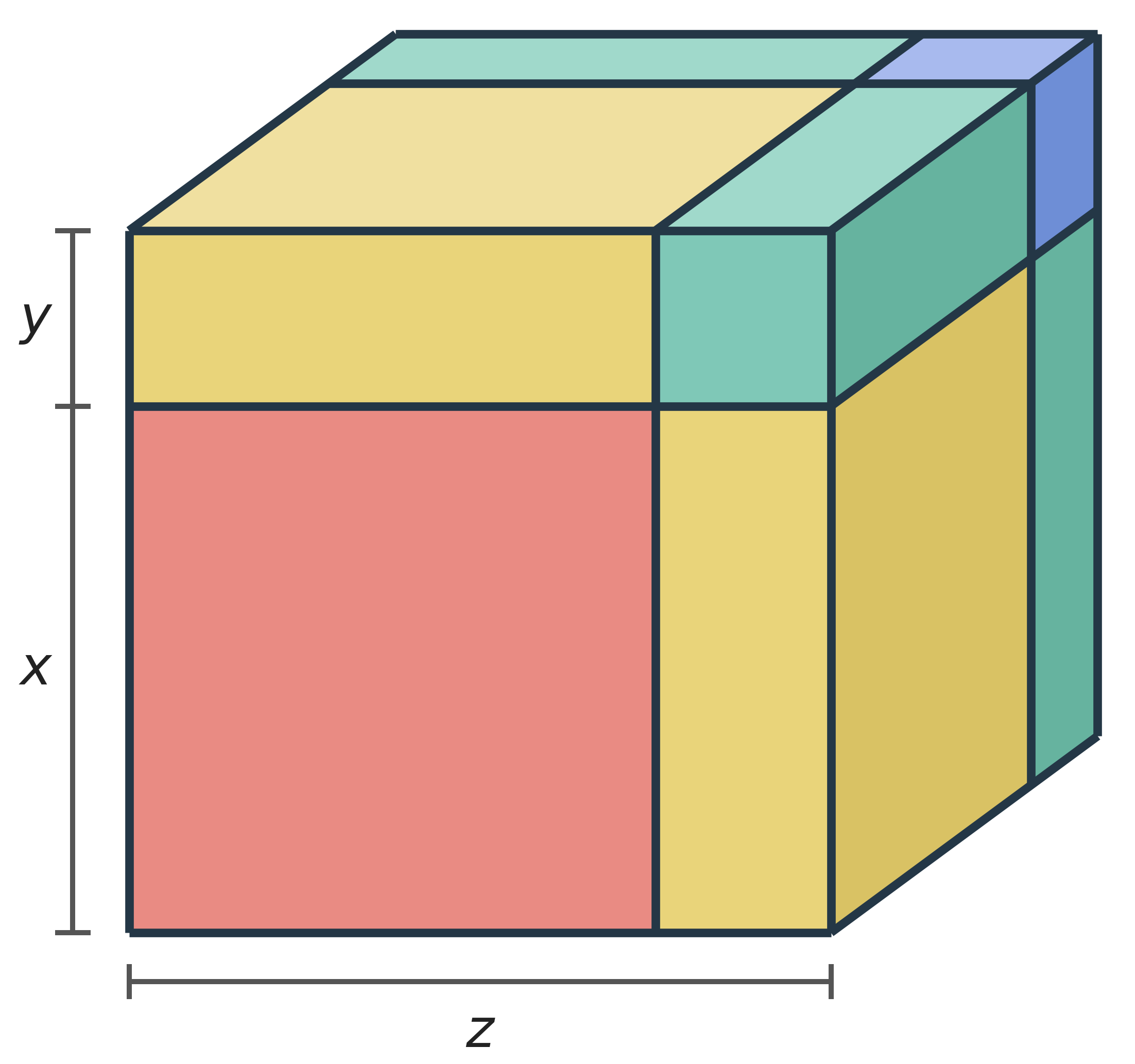
This larger cube is composed of eight shapes:

• The original cube with side lengths of \(x\), and volume \(x^{3}\)

• three rectangular prisms with dimensions \(x\) by \(x\) by \(y\), and total volume \(3x^{2}y\)

• three more prisms with dimensions \(x\) by \(y\) by \(y\), and total volume \(3xy^{2}\)

• A smaller cube with side length \(y\), and volume \(y^{3}\)

Algebraically, this is equivalent to expressing \(z\) as \(x + y\) and expanding out the expression:

\[{(x + y)}^{3} = x^{3} + 3x^{2}y + 3xy^{2} + y^{3}\]

Figure 2.2

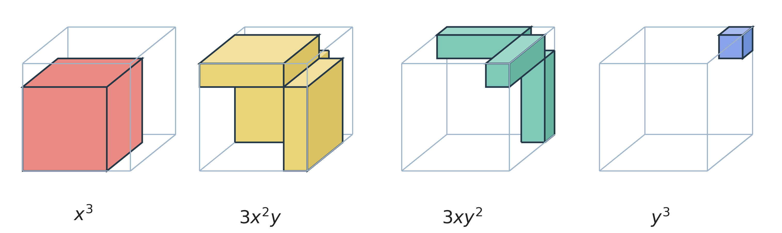
The volume of the cube is the exact same as the terms in the algebraic expansion.

Now, we want a portion of the extra volume to match up with our linear term, \(3x\). Geometrically, we can combine the two sets of three prisms each into one block, with a volume of \(3yzx\). This matches up with our linear term.

Figure 2.3

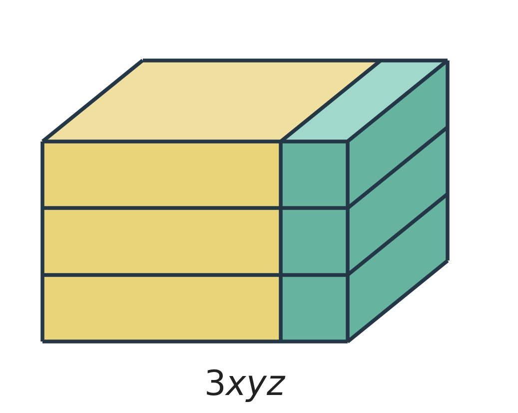
Algebraically, we can factor out \(3yx\) from the middle terms, giving

\[z^{3} = x^{3} + 3yx(x + y) + y^{3}\]

Because \(z = x + y\), now we have

\[z^{3}{= x}^{3} + 3yzx + y^{3}\]

Now the middle term can perfectly match up with the \(3x\) term in our equation, so we get the same equation as before, and can match the terms like this.

Figure 2.4

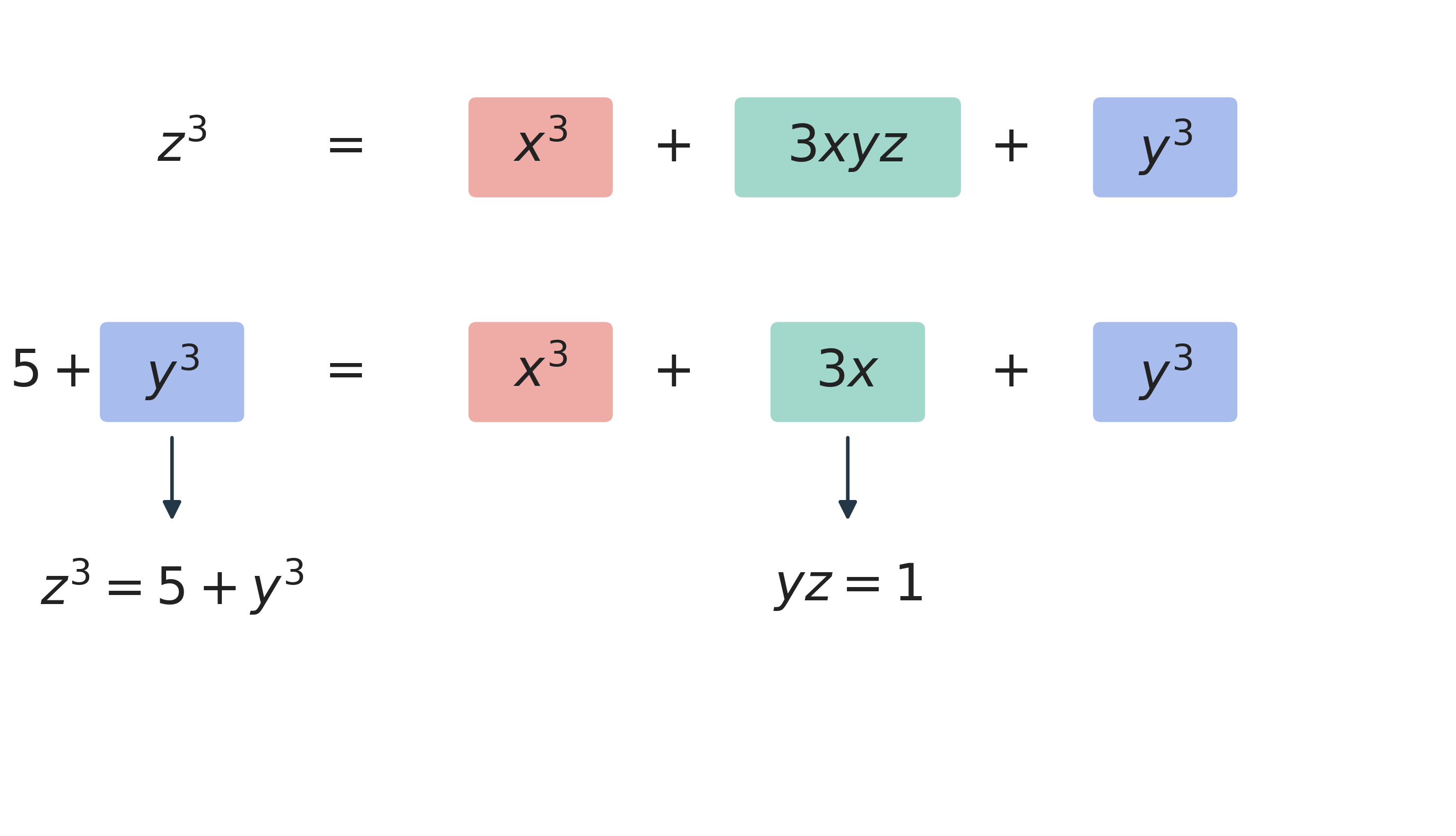
So now we have the equation \(3yz = 3\). All we need to do now is add \(y^{3}\) to both sides to “complete the cube”. So now we have

\[z^{3} = 5 + y^{3}\]

We have two equations and two unknowns: \(\left\{\begin{aligned} 3yz &= 3 \\ z^{3} &= 5 + y^{3} \end{aligned}\right.\)

In the first equation we can divide through by \(3y\), giving us

\[z = \frac{1}{y}\]

We can now substitute this into the second equation to have only one variable:

\[\frac{1}{y^{3}} = 5 + y^{3}\]

Multiplying through by \(y^{3}\), we obtain the equation

\[1 = 5y^{3} + y^{6}\]

At first, it looks like we have gone from bad to worse, since now we have a sixth power term in the equation. But this equation is really a quadratic in disguise, because

\[1 = 5y^{3} + {(y^{3})}^{2}\]

We can now complete the square as before!!

We add \(\frac{25}{4}\) to both sides to complete the square,

\[{(y^{3})}^{2} + 5y^{3} + \frac{25}{4} = \frac{29}{4}\]

Therefore

\[{(y^{3} + \frac{5}{2})}^{2} = \frac{29}{4}\]

Taking the square root of both sides:

\[y^{3} + \frac{5}{2} = \pm \frac{\sqrt{29}}{2}\]

Our final answer is that

\[y = \sqrt[3]{\frac{- 5 \pm \sqrt{29}}{2}}\]

We will deal with the plus minus later.

Now we need to solve for \(z\), which is easily done by plugging into \(z^{3} = 5 + y^{3}\).

\[z^{3} = 5 + \left( \frac{- 5 \pm \sqrt{29}}{2} \right)\]

After simplifying, we find

\[z^{3} = \frac{5 \pm \sqrt{29}}{2}\]

Now we can isolate \(z\) by taking the cube root.

\[z = \sqrt[3]{\frac{5 \pm \sqrt{29}}{2}}\]

We have known from the start that \(x + y = z\). Therefore, \(x = z - y\).

By substitution,

\[x = \sqrt[3]{\frac{5 \pm \sqrt{29}}{2}} - \sqrt[3]{\frac{- 5 \pm \sqrt{29}}{2}}\]

Distributing the minus sign in the cube root gives our solution:

\[x = \sqrt[3]{\frac{5 \pm \sqrt{29}}{2}} + \sqrt[3]{\frac{5 \mp \sqrt{29}}{2}}\]

Notice how the minus sign has turned the plus/minus into a minus/plus. This negation means that the cube roots must have opposite signs on the plus/minus sign, leaving us with one solution:

\[x = \sqrt[3]{\frac{5 + \sqrt{29}}{2}} + \sqrt[3]{\frac{5 - \sqrt{29}}{2}}\]

Amazing!

So \(x \approx 1.1542\), and you can check that this is a solution. This is also the only real solution.

Depressing the Cubic

But what about an equation like \(x^{3} + 2x^{2} + 5x = 7\)? We can’t employ the same trick with completing the cube, but Cardano figured out how to turn this equation into a depressed cubic that can be solved like before. The technique is to substitute a new variable related to \(x\), in a specific way such that the original equation is turned into a depressed cubic, which we can solve.

The general technique is to substitute in the variable, \(\boxed{x = w - \frac{b}{3a}}\), which will always reduce to a depressed cubic in terms of \(w\).

In our example, we substitute \(x = w - \frac{2}{3}\), then we can plug in and find that the quadratic terms cancel out:

\[\left( w - \frac{2}{3} \right)^{3} + 2\left( w - \frac{2}{3} \right)^{2} + 5\left( w - \frac{2}{3} \right) = 7\]

Expanding:

\[w^{3} - 2w^{2} + \frac{4}{3}w - \frac{8}{27} + 2w^{2} - \frac{8}{3}w + \frac{8}{9} + 5w - \frac{10}{3} = 7\]

After combining like terms, we get a depressed cubic:

\[w^{3} + \frac{11}{3}w = \frac{263}{27}\]

We can solve this equation with the same method as above.

We can extend the cube with side lengths \(w\) by a length \(y\), making a larger cube with side length \(z\).

Figure 2.5

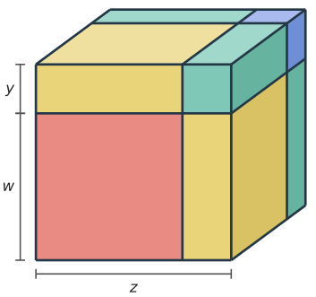
Now, rearranging the blocks geometrically or factoring algebraically provides

\[z^{3} = w^{3} + 3yzw + y^{3}\]

Matching terms, we get the equation \(3yz = \frac{11}{3}\).

Now, we can add \(y^{3}\) to both sides in our original equation to find: \(z^{3} = \frac{263}{27} + y^{3}\)

Now we have a similar system of equations: \(\left\{\begin{aligned} 3yz &= \frac{11}{3} \\ z^{3} &= \frac{263}{27} + y^{3} \end{aligned}\right.\)

Solving the first equation for \(z\):

\[z = \frac{11}{9y}\]

Substituting into the second equation:

\[\left( \frac{11}{9y} \right)^{3} = \frac{263}{27} + y^{3}\]

Simplifying:

\[\frac{1331}{729y^{3}} = \frac{263}{27} + y^{3}\]

Multiplying by \(y^{3}\) to get a quadratic:

\[\frac{1331}{729} = \left( y^{3} \right)^{2} + \frac{263}{27}y^{3}\]

Now we can solve by completing the square, as usual.

We add \(\frac{69169}{2916}\) , which is the square of half the linear coefficient, to both sides to complete the square:

\[\left( y^{3} \right)^{2} + \frac{263}{27}y^{3} + \frac{69169}{2916} = \frac{2759}{108}\]

Folding into a perfect square and simplifying:

\[\left( y^{3} + \frac{263}{54} \right)^{2} = \frac{2759}{108}\]

Now we can solve for \(y\) in a couple of steps:

\[y^{3} + \frac{263}{54} = \pm \frac{\sqrt{8277}}{18}\]

\[y^{3} = \frac{- 263 \pm 3\sqrt{8277}}{54}\]

\[y = \sqrt[3]{\frac{- 263 \pm 3\sqrt{8277}}{54}\ }\]

Now we can solve for \(z\) by plugging into the second equation:

\[z^{3} = \frac{263}{27} + \frac{- 263 \pm 3\sqrt{8277}}{54}\]

Simplifying:

\[z^{3} = \frac{263 \pm 3\sqrt{8277}}{54}\]

Isolating \(z\) by cube roots:

\[z = \sqrt[3]{\frac{263 \pm 3\sqrt{8277}}{54}\ }\]

Now we know from the starting equation \(w + y = z\), so equivalently \(w = z - y\).

\[w = \sqrt[3]{\frac{263 \pm 3\sqrt{8277}}{54}\ } + \sqrt[3]{\frac{263 \mp 3\sqrt{8277}}{54}\ }\]

The only solution that works is when the roots have opposing plus/minus signs; therefore

\[w = \sqrt[3]{\frac{263 + 3\sqrt{8277}}{54}} + \sqrt[3]{\frac{263 - 3\sqrt{8277}}{54}}\]

The actual variable we were looking for was \(x\), which we can easily find by remembering that \(x = w - \frac{2}{3}\), so we can substitute for \(x\):

\[x = \sqrt[3]{\frac{263 + 3\sqrt{8277}}{54}} + \sqrt[3]{\frac{263 - 3\sqrt{8277}}{54}} - \frac{2}{3}\]

Our approximate value is \(x \approx 0.9136\).

The General Cubic Formula

I will now present a derivation of the cubic formula in the general case, using letters instead of numbers for the coefficients. The techniques to solve it are the exact same as discussed before.

We start with the general cubic equation:

\[ax^{3} + bx^{2} + cx + d = 0\]

Here the coefficients are real and \(a\) is not \(0\). We can divide by \(a\) to simplify one of the coefficients, so we get

\[x^{3} + \frac{b}{a}x^{2} + \frac{c}{a}x + \frac{d}{a} = 0\]

Now we can employ Cardano’s substitution to get rid of the quadratic term. In the general case, we substitute \(x = w - \frac{b}{3a}\).

\[\left( w - \frac{b}{3a} \right)^{3} + \frac{b}{a}\left( w - \frac{b}{3a} \right)^{2} + \frac{c}{a}\left( w - \frac{b}{3a} \right) + \frac{d}{a} = 0\]

The expansion gets messy and is very dull, so think of it as algebra autopilot.

\[\left( w^{3} - \frac{b}{a}w^{2} + \frac{b^{2}}{3a^{2}}w - \frac{b^{3}}{27a^{3}} \right) + \frac{b}{a}\left( w^{2} - \frac{2b}{3a}w + \frac{b^{2}}{9a^{2}} \right) + \frac{c}{a}\left( w - \frac{b}{3a} \right) + \frac{d}{a} = 0\]

Now we distribute into the parentheses (sigh!)

\[w^{3} - \frac{b}{a}w^{2} + \frac{b^{2}}{3a^{2}}w - \frac{b^{3}}{27a^{3}} + \frac{b}{a}w^{2} - \frac{2b^{2}}{3a^{2}}w + \frac{b^{3}}{9a^{3}} + \frac{c}{a}w - \frac{bc}{3a^{2}} + \frac{d}{a} = 0\]

Now, combining all like terms, we find that the quadratic terms have cancelled!

\[w^{3} + \left( - \frac{b^{2}}{3a^{2}} + \frac{c}{a} \right)w + \left( \frac{2b^{3}}{27a^{3}} - \frac{bc}{3a^{2}} + \frac{d}{a} \right) = 0\]

To simplify things, I will call the new coefficients \(p\) and \(q\).

\[p = - \frac{b^{2}}{3a^{2}} + \frac{c}{a},\ q = + \frac{2b^{3}}{27a^{3}} - \frac{bc}{3a^{2}} + \frac{d}{a}\]

Now we have the depressed cubic \(w^{3} + pw + q = 0\), which we can solve by completing the cube.

The picture uses positive lengths; the algebraic identities also hold for signed values. Visualizing \(w^{3}\) as an actual cube, we add on a distance \(y\) in all three directions, making a larger cube with dimensions of \(z\).

Algebraically, we expand out like so: \(z^{3} = w^{3} + 3yw^{2} + 3y^{2}w + y^{3}\).

Geometrically, we rearrange the outside blocks to form a single composite block with dimensions \(3y\) by \(w + y\) by \(w\).

See Figure 2.5.

Algebraically, we can factor out \(3wy\) from the middle terms to get

\[z^{3} = w^{3} + 3wy(w + y) + y^{3}\]

Remember that \(z = w + y\); then

\[z^{3} = w^{3} + 3yzw + y^{3}\]

We now know that \(p = 3yz\) from matching terms. To “complete the cube”, we must add \(y^{3}\) to both sides of the equation \(w^{3} + 3yzw + q = 0\). So our equation becomes \(z^{3} + q = y^{3}\)

And now we have a system of equations in terms of \(y\) and \(z\), our unknowns:

\[\left\{\begin{aligned} p &= 3yz \\ z^{3} + q &= y^{3} \end{aligned}\right.\]

If \(p\) is \(0\), the depressed equation is solved directly by taking the real cube root of \(- q\). Otherwise, \(p = 3yz\) means \(y\) cannot be \(0\), so we can solve for \(z\) in the first equation:

\[\frac{p}{3y} = z\]

Now we can substitute into the second equation:

\[\frac{p^{3}}{27y^{3}} + q = y^{3}\]

Multiplying through by \(y^{3}\), we get the quadratic equation:

\[\frac{p^{3}}{27}{{+ qy^{3} = (y}^{3})}^{2}\]

Moving terms, we get it into standard form:

\[{{(y}^{3})}^{2} - qy^{3} - \frac{p^{3}}{27} = 0\]

Solving using the quadratic formula, we get

\[y^{3} = \frac{q \pm \sqrt{q^{2} + \frac{4p^{3}}{27}}}{2}\]

We can now clean up the right side by distributing the fraction into the square root like this:

\[y^{3} = \frac{q}{2} \pm \sqrt{\frac{1}{4}}*\sqrt{q^{2} + \frac{4p^{3}}{27}}\]

We can use properties of radicals to simplify

\[y^{3} = \frac{q}{2} \pm \sqrt{\frac{q^{2}}{4} + \frac{p^{3}}{27}}\]

We can factor inside the square root to get

\[y^{3} = \frac{q}{2} \pm \sqrt{\left( \frac{q}{2} \right)^{2} + \left( \frac{p}{3} \right)^{3}}\]

Finally, we can get \(y\) in terms of \(p\) and \(q\)!

\[y = \sqrt[3]{\frac{q}{2} \pm \sqrt{\left( \frac{q}{2} \right)^{2} + \left( \frac{p}{3} \right)^{3}}}\]

When the square root is real and we use real cube roots, it doesn’t matter if we choose the plus or minus value of \(y\), as it will work out to the same formula in the end. By convention, I will usually choose the plus sign, though using the minus sign works just fine as well!

Plugging \(y\) into equation 2 yields:

\[z^{3} + q = \frac{q}{2} + \sqrt{\left( \frac{q}{2} \right)^{2} + \left( \frac{p}{3} \right)^{3}}\]

Moving \(q\) to the opposite side:

\[z^{3} = - \frac{q}{2} + \sqrt{\left( \frac{q}{2} \right)^{2} + \left( \frac{p}{3} \right)^{3}}\]

Therefore

\[z = \sqrt[3]{- \frac{q}{2} + \sqrt{\left( \frac{q}{2} \right)^{2} + \left( \frac{p}{3} \right)^{3}}}\]

Assuming the plus/minus sign is a minus gives the same solution.

We know that \(w + y = z\), so \(w = z - y\). Substituting in,

\[\begin{aligned} w &= \sqrt[3]{- \frac{q}{2} + \sqrt{\left( \frac{q}{2} \right)^{2} + \left( \frac{p}{3} \right)^{3}}} \\ &\quad - \sqrt[3]{\frac{q}{2} + \sqrt{\left( \frac{q}{2} \right)^{2} + \left( \frac{p}{3} \right)^{3}}} \end{aligned}\]

Only the opposing signs version will produce a suitable solution, so our formula for depressed cubic equations is

\[w = \sqrt[3]{- \frac{q}{2} + \sqrt{\left( \frac{q}{2} \right)^{2} + \left( \frac{p}{3} \right)^{3}}} + \sqrt[3]{- \frac{q}{2} - \sqrt{\left( \frac{q}{2} \right)^{2} + \left( \frac{p}{3} \right)^{3}}}\]

To find our original solutions, we simply need to back substitute for \(p\), \(q\) and \(w\). This will get very messy just for the moment, but everything will simplify. Remember,

\[p = - \frac{b^{2}}{3a^{2}} + \frac{c}{a}\text{, }q = + \frac{2b^{3}}{27a^{3}} - \frac{bc}{3a^{2}} + \frac{d}{a}\]

\[\begin{aligned} w &= \sqrt[3]{\frac{- \left( + \frac{2b^{3}}{27a^{3}} - \frac{bc}{3a^{2}} + \frac{d}{a} \right)}{2} + \sqrt{\left( \frac{\left( + \frac{2b^{3}}{27a^{3}} - \frac{bc}{3a^{2}} + \frac{d}{a} \right)}{2} \right)^{2} + \left( \frac{\left( - \frac{b^{2}}{3a^{2}} + \frac{c}{a} \right)}{3} \right)^{3}}} \\ &\quad + \sqrt[3]{\frac{- ( + \frac{2b^{3}}{27a^{3}} - \frac{bc}{3a^{2}} + \frac{d}{a})}{2} - \sqrt{\left( \frac{( + \frac{2b^{3}}{27a^{3}} - \frac{bc}{3a^{2}} + \frac{d}{a})}{2} \right)^{2} + \left( \frac{- \frac{b^{2}}{3a^{2}} + \frac{c}{a}}{3} \right)^{3}}} \end{aligned}\]

This looks awful, but dividing everything out makes it much cleaner:

\[w = \sqrt[3]{- \frac{b^{3}}{27a^{3}} + \frac{bc}{6a^{2}} - \frac{d}{2a} + \sqrt{\left( \frac{b^{3}}{27a^{3}} - \frac{bc}{6a^{2}} + \frac{d}{2a} \right)^{2} + \left( - \frac{b^{2}}{9a^{2}} + \frac{c}{3a} \right)^{3}}}\]

\[+ \sqrt[3]{- \frac{b^{3}}{27a^{3}} + \frac{bc}{6a^{2}} - \frac{d}{2a} - \sqrt{\left( \frac{b^{3}}{27a^{3}} - \frac{bc}{6a^{2}} + \frac{d}{2a} \right)^{2} + \left( - \frac{b^{2}}{9a^{2}} + \frac{c}{3a} \right)^{3}}}\]

We are almost there! Since \(x = w - \frac{b}{3a}\), all we have to do now is subtract \(\frac{b}{3a}\) from the expression!

Finally, after all this work, our final formula is…

\[x = \sqrt[3]{- \frac{b^{3}}{27a^{3}} + \frac{bc}{6a^{2}} - \frac{d}{2a} + \sqrt{\left( \frac{b^{3}}{27a^{3}} - \frac{bc}{6a^{2}} + \frac{d}{2a} \right)^{2} + \left( - \frac{b^{2}}{9a^{2}} + \frac{c}{3a} \right)^{3}}}\] \[+ \sqrt[3]{- \frac{b^{3}}{27a^{3}} + \frac{bc}{6a^{2}} - \frac{d}{2a} - \sqrt{\left( \frac{b^{3}}{27a^{3}} - \frac{bc}{6a^{2}} + \frac{d}{2a} \right)^{2} + \left( - \frac{b^{2}}{9a^{2}} + \frac{c}{3a} \right)^{3}}} - \frac{b}{3a}\]

This is the general cubic formula!

When the square root is real, real cube roots give us a real solution. Repeated roots and negative numbers under the square root need some extra care, as we will see shortly.

Completing the Cube, Extended

There is another method to arrive at this formula, which extends completing the cube to the general cubic without having to use Cardano’s substitution. I developed this method independently, and I don’t know whether this exact derivation has appeared before.¹²

For simplicity, I will assume \(a = 1\) for now, so we have the equation \(x^{3} + bx^{2} + cx + d = 0\). Any general cubic equation can be made into this form through dividing by \(a\).

Again, the picture uses positive lengths; the algebraic identities also hold for signed values. Now we can start with the cube we have constructed before, the one with a side length of \(x + y\). The trick here is to use this cube as the basis to complete the cube again. We can extend this large cube a distance of \(u\) in all directions. This creates a cube with side length \(x + y + u\), which I will call a distance of \(v\). Therefore, \(x + y + u = v\).

Figure 2.6

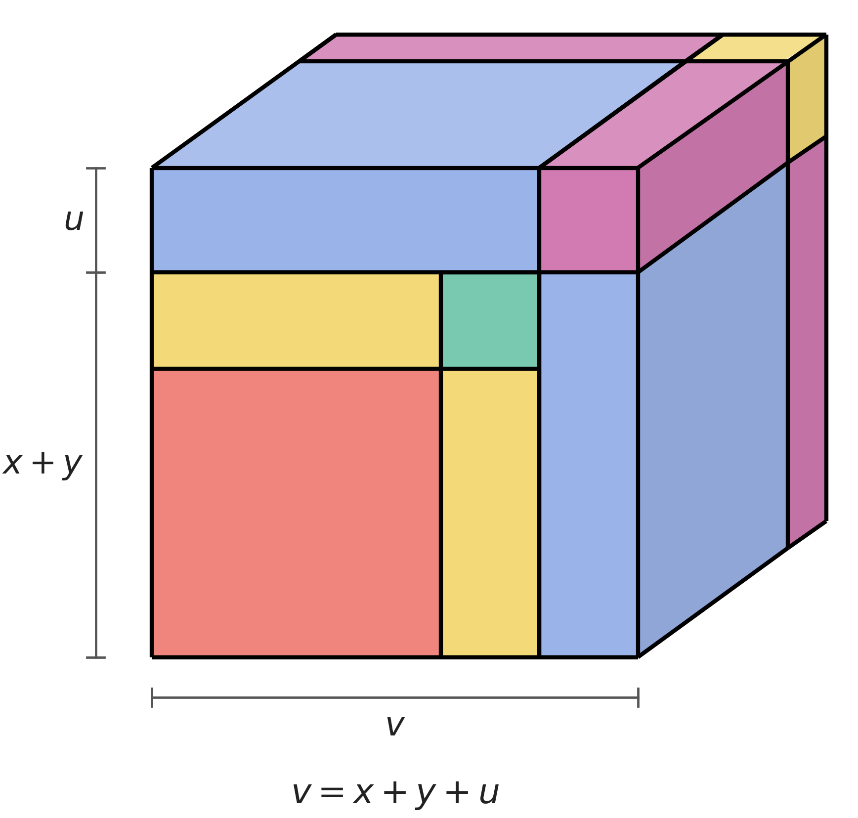
The total new volume, including the original \(x + y\) cube, is made up of eight shapes

• The original \(x + y\) cube, with volume \((x + y)^{3}\)

• three rectangular prisms with dimensions of \((x + y)\) by \((x + y)\) by \(u\)

• three more prisms with dimensions \((x + y)\) by \(u\) by \(u\)

• A small cube \(u^{3}\)

Figure 2.7

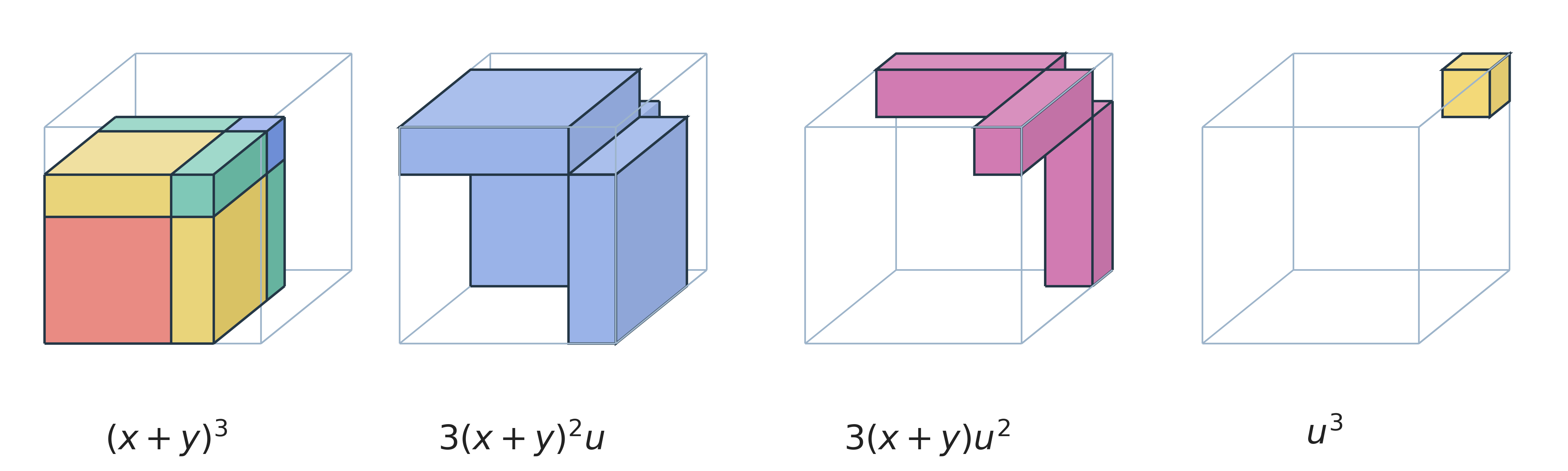
This is equivalent to algebraically expanding out \({(x + y + u)}^{3}\).

We treat \((x + y)\) as a single number, and expand \({(x + y)}^{3} + 3u{(x + y)}^{2} + 3u^{2}(x + y) + u^{3}\).

The next step is to break apart the two sets of prisms into smaller blocks.

With the larger prisms, since the sides are length \((x + y)\), we can divide one side into one segment with length \(x\) and the other with length \(y\). Doing this for each prism yields three blocks with dimensions \((x + y)\) by \(x\) by \(u\) and three more blocks with dimensions \((x + y)\) by \(y\) by \(u\). I will refer to these as “x blocks” and “y blocks” for clarity.

In a similar manner, we can break apart the narrower prisms in the same way, making three prisms with dimensions \(u\) by \(x\) by \(u\), our “x blocks”, and three more with dimensions \(u\) by \(y\) by \(u\), our “y blocks”.

Figure 2.8

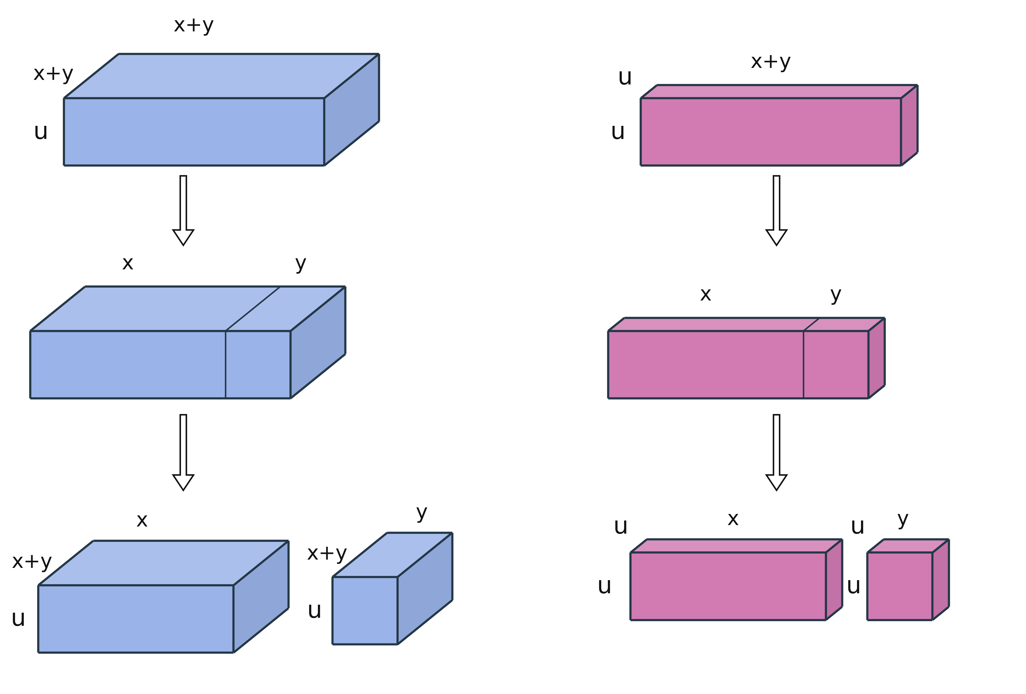
Algebraically, this is the same as expanding the \((x + y)\) in the middle terms:

\[{(x + y)}^{3} + 3ux(x + y) + 3uy(x + y) + 3u^{2}x + 3u^{2}y + u^{3}\text{. }\]

The next step is to combine the three sets of x blocks and y blocks, creating three combined x blocks measuring \((x + y + u)\) by \(x\) by \(u\), and three combined y blocks measuring \((x + y + u)\) by \(y\) by \(u\).

Algebraically this is equivalent to factoring either \(3ux\) or \(3uy\) out of all middle terms and grouping \({(x + y)}^{3} + 3ux(x + y) + 3ux(u) + 3uy(x + y) + 3uy(u) + u^{3}\). Now we can group like terms \((x + y)^{3} + 3ux(x + y + u) + 3uy(x + y + u) + u^{3}\). Finally, we recognize that \(v = x + y + u\), so we can substitute \({(x + y)}^{3} + 3uvx + 3uvy + u^{3}\).

Figure 2.9

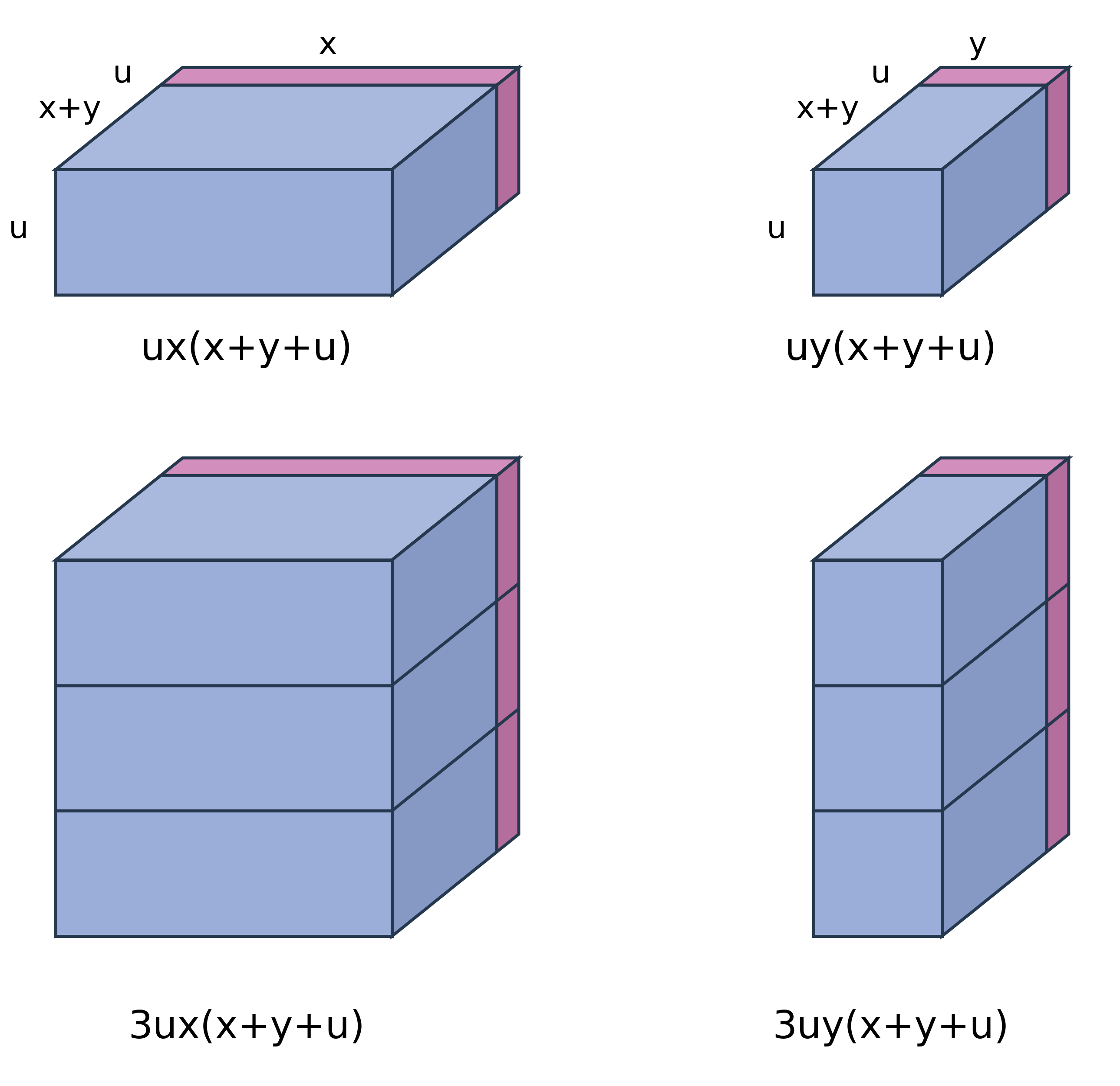
Now, our final step is to decompose the \(x + y\) cube into the shapes we have seen before:

Geometrically, our complete shapes list is:

• The original cube with side length \(x\), volume \(x^{3}\)

• three prisms with dimensions \(x\) by \(x\) by \(y\), total volume \(3yx^{2}\)

• three prisms with dimensions \(x\) by \(y\) by \(y\), total volume \(3y^{2}x\)

• three prisms with dimensions \(u\) by \(v\) by \(x\), total volume \(3uvx\)

• three prisms with dimensions \(u\) by \(v\) by \(y\), total volume \(3uvy\)

• A cube with side length \(y\), volume \(y^{3}\)

• A cube with side length \(u\), volume \(u^{3}\)

In algebraic terms, we simply expand out \({(x + y)}^{3}\): \(v^{3} = x^{3} + 3yx^{2} + 3y^{2}x + y^{3} + 3uvx + 3uvy + u^{3}\).

Figure 2.10

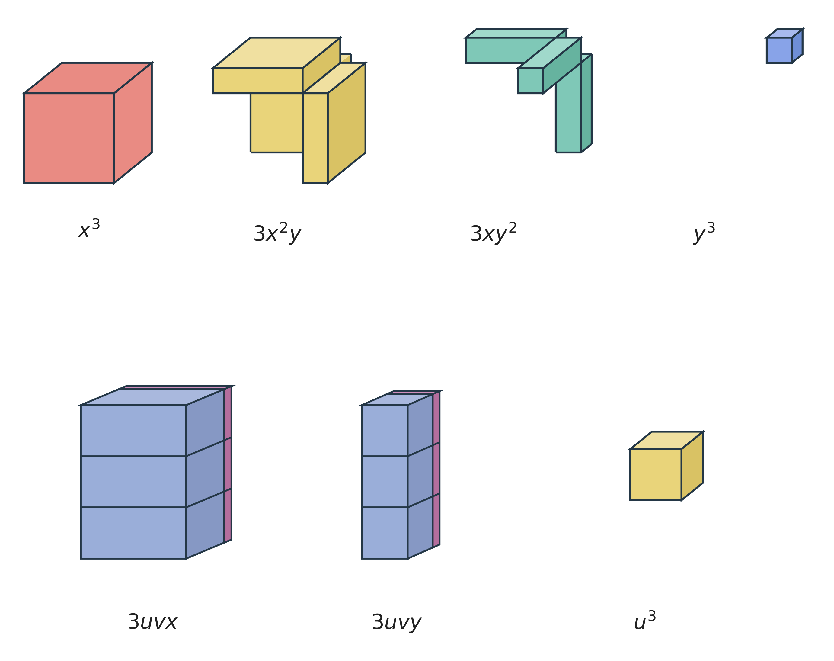
Now we can group terms according to powers of \(x\): \(v^{3} = x^{3} + 3yx^{2} + \left( 3y^{2} + 3uv \right)x + (y^{3} + u^{3} + 3uvy)\).

This looks promising, as now we can match up both the quadratic and linear terms to our original equation:

Figure 2.11

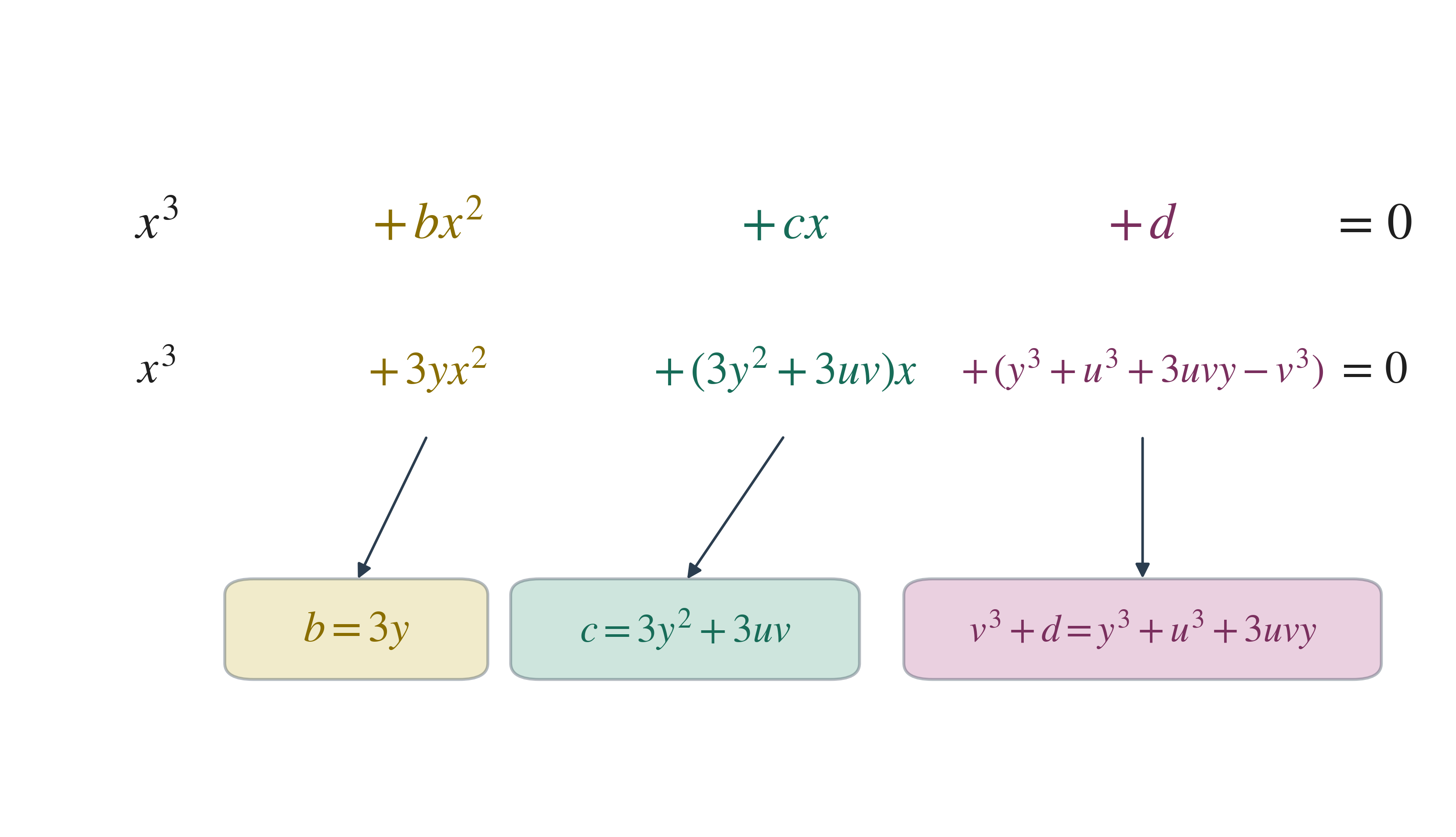
This gives us two equations: \(\left\{\begin{aligned} b &= 3y \\ c &= 3y^{2} + 3uv \end{aligned}\right.\)

To “complete the cube” in this case, we need to add on all three constant terms to both sides:

This gives us our third equation: \(v^{3} + d = y^{3} + u^{3} + 3uvy\).

Now we have a system of three equations in three variables:

\[\left\{\begin{aligned} b &= 3y \\ c &= 3y^{2} + 3uv \\ v^{3} + d &= y^{3} + u^{3} + 3uvy \end{aligned}\right.\]

Fortunately, the first equation is easy to solve, showing \(y = \frac{b}{3}\).

Now we can substitute this into the second and third equations: \(\left\{\begin{aligned} c &= 3\left( \frac{b}{3} \right)^{2} + 3uv \\ v^{3} + d &= \left( \frac{b}{3} \right)^{3} + u^{3} + 3uvy \end{aligned}\right.\).

Now let’s simplify the second equation: \(c = \frac{b^{2}}{3} + 3uv\).

If \(c = \frac{b^{2}}{3}\), we use the zero-linear-coefficient case from the previous method. Otherwise \(u\) cannot be \(0\), and we can solve for \(v\) in a couple of steps:

\[c - \frac{b^{2}}{3} = 3uv\]

Therefore

\[v = \frac{\frac{c}{3} - \frac{b^{2}}{9}}{u}\]

Now, we can plug this result into our third equation, and simplify:

\[\left( \frac{\frac{c}{3} - \frac{b^{2}}{9}}{u} \right)^{3} + d = \frac{b^{3}}{27} + u^{3} + 3uvy\]

The only term left is \(3uvy\). We can substitute in \(3uv = c - \frac{b^{2}}{3}\) and \(y = \frac{b}{3}\) to get an equation only in \(u\):

\[\frac{\left( \frac{c}{3} - \frac{b^{2}}{9} \right)^{3}}{u^{3}} + d = u^{3} + \frac{b^{3}}{27} + \left( c - \frac{b^{2}}{3} \right)\left( \frac{b}{3} \right)\]

We can group all constants together and simplify:

\[\frac{\left( \frac{c}{3} - \frac{b^{2}}{9} \right)^{3}}{u^{3}} = u^{3} - \frac{2b^{3}}{27} + \frac{bc}{3} - d\]

Multiplying through by the cube of \(u\) gives us a disguised quadratic:

\[\left( \frac{c}{3} - \frac{b^{2}}{9} \right)^{3} = \left( u^{3} \right)^{2} + \left( - \frac{2b^{3}}{27} + \frac{bc}{3} - d \right)u^{3}\]

To apply the quadratic formula, we move everything to one side:

\[0 = \left( u^{3} \right)^{2} + \left( - \frac{2b^{3}}{27} + \frac{bc}{3} - d \right)u^{3} - \left( \frac{c}{3} - \frac{b^{2}}{9} \right)^{3}\]

Now we use the quadratic formula to solve for \(u^{3}\):

\[u^{3} = \frac{- \left( - \frac{2b^{3}}{27} + \frac{bc}{3} - d \right) \pm \sqrt{\left( - \frac{2b^{3}}{27} + \frac{bc}{3} - d \right)^{2} + 4\left( \frac{c}{3} - \frac{b^{2}}{9} \right)^{3}}}{2}\]

Now we simplify the fractions:

\[u^{3} = \frac{b^{3}}{27} - \frac{bc}{6} + \frac{d}{2} \pm \frac{\sqrt{\left( - \frac{2b^{3}}{27} + \frac{bc}{3} - d \right)^{2} + 4\left( \frac{c}{3} - \frac{b^{2}}{9} \right)^{3}}}{2}\]

Next, we use properties of square roots to rewrite the fraction:

\[u^{3} = \frac{b^{3}}{27} - \frac{bc}{6} + \frac{d}{2} \pm \sqrt{\frac{1}{4}}*\sqrt{\left( - \frac{2b^{3}}{27} + \frac{bc}{3} - d \right)^{2} + 4\left( \frac{c}{3} - \frac{b^{2}}{9} \right)^{3}}\]

Now, we divide everything inside the square root by \(4\):

\[u^{3} = \frac{b^{3}}{27} - \frac{bc}{6} + \frac{d}{2} \pm \sqrt{\frac{\left( - \frac{2b^{3}}{27} + \frac{bc}{3} - d \right)^{2}}{4} + \left( \frac{c}{3} - \frac{b^{2}}{9} \right)^{3}}\]

Now we rewrite \(4\) as \(2^{2}\), and divide everything in the expression by \(2\):

\[u^{3} = \frac{b^{3}}{27} - \frac{bc}{6} + \frac{d}{2} \pm \sqrt{\left( - \frac{b^{3}}{27} + \frac{bc}{6} - \frac{d}{2} \right)^{2} + \left( \frac{c}{3} - \frac{b^{2}}{9} \right)^{3}}\]

Finally, we take the cube root to isolate \(u\):

\[u = \sqrt[3]{\frac{b^{3}}{27} - \frac{bc}{6} + \frac{d}{2} \pm \sqrt{\left( - \frac{b^{3}}{27} + \frac{bc}{6} - \frac{d}{2} \right)^{2} + \left( \frac{c}{3} - \frac{b^{2}}{9} \right)^{3}}}\]

As before, when the square root is real and we use real cube roots, it doesn’t matter if \(u\) has the plus or minus solution. By convention, I will choose the plus.

To isolate \(v\), we plug in our results for \(u\) into the altered third equation

\[v^{3} + d = u^{3} - \frac{2b^{3}}{27} + \frac{bc}{3}\]

This version was obtained by substituting in for \(y\) and \(3uv\), but not for \(v^{3}\).

By substitution:

\[v^{3} + d = \frac{b^{3}}{27} - \frac{bc}{6} + \frac{d}{2} + \sqrt{\left( - \frac{b^{3}}{27} + \frac{bc}{6} - \frac{d}{2} \right)^{2} + \left( \frac{c}{3} - \frac{b^{2}}{9} \right)^{3}} - \frac{2b^{3}}{27} + \frac{bc}{3}\]

After moving all constants to the right and combining like terms:

\[v^{3} = - \frac{b^{3}}{27} + \frac{bc}{6} - \frac{d}{2} + \sqrt{\left( - \frac{b^{3}}{27} + \frac{bc}{6} - \frac{d}{2} \right)^{2} + \left( \frac{c}{3} - \frac{b^{2}}{9} \right)^{3}}\]

Now we can isolate \(v\):

\[v = \sqrt[3]{- \frac{b^{3}}{27} + \frac{bc}{6} - \frac{d}{2} + \sqrt{\left( - \frac{b^{3}}{27} + \frac{bc}{6} - \frac{d}{2} \right)^{2} + \left( \frac{c}{3} - \frac{b^{2}}{9} \right)^{3}}}\]

Now that we have solved for \(y\), \(u\) and \(v\), we can use the equation \(x + y + u = v\) to get \(x\). By moving terms, \(x = v - u - y\).

Plugging into the expression above, we get this formula for \(x\):

\[\begin{aligned} &x = \sqrt[3]{- \frac{b^{3}}{27} + \frac{bc}{6} - \frac{d}{2} + \sqrt{\left( - \frac{b^{3}}{27} + \frac{bc}{6} - \frac{d}{2} \right)^{2} + \left( \frac{c}{3} - \frac{b^{2}}{9} \right)^{3}}} \\[1.1em] &\quad - \sqrt[3]{\frac{b^{3}}{27} - \frac{bc}{6} + \frac{d}{2} + \sqrt{\left( - \frac{b^{3}}{27} + \frac{bc}{6} - \frac{d}{2} \right)^{2} + \left( \frac{c}{3} - \frac{b^{2}}{9} \right)^{3}}} - \frac{b}{3}\text{. } \end{aligned}\]

We can distribute the minus sign into the second cube root, making:

\[\begin{aligned} &x = \sqrt[3]{- \frac{b^{3}}{27} + \frac{bc}{6} - \frac{d}{2} + \sqrt{\left( - \frac{b^{3}}{27} + \frac{bc}{6} - \frac{d}{2} \right)^{2} + \left( \frac{c}{3} - \frac{b^{2}}{9} \right)^{3}}} \\[1.1em] &\quad + \sqrt[3]{- \frac{b^{3}}{27} + \frac{bc}{6} - \frac{d}{2} - \sqrt{\left( - \frac{b^{3}}{27} + \frac{bc}{6} - \frac{d}{2} \right)^{2} + \left( \frac{c}{3} - \frac{b^{2}}{9} \right)^{3}}} - \frac{b}{3} \end{aligned}\]

In addition, we assumed \(a = 1\) at the beginning, so this formula isn’t completely general. This is remedied by replacing \(b\) with \(\frac{b}{a}\); \(c\) with \(\frac{c}{a}\); and \(d\) with \(\frac{d}{a}\), because you can always divide by \(a\) before you start solving. Therefore, our final formula is:

\[x = \sqrt[3]{- \frac{b^{3}}{27a^{3}} + \frac{bc}{6a^{2}} - \frac{d}{2a} + \sqrt{\left( \frac{b^{3}}{27a^{3}} - \frac{bc}{6a^{2}} + \frac{d}{2a} \right)^{2} + \left( - \frac{b^{2}}{9a^{2}} + \frac{c}{3a} \right)^{3}}}\]

\[+ \sqrt[3]{- \frac{b^{3}}{27a^{3}} + \frac{bc}{6a^{2}} - \frac{d}{2a} - \sqrt{\left( \frac{b^{3}}{27a^{3}} - \frac{bc}{6a^{2}} + \frac{d}{2a} \right)^{2} + \left( - \frac{b^{2}}{9a^{2}} + \frac{c}{3a} \right)^{3}}} - \frac{b}{3a}\]

This is the exact same result we got before, but derived differently.

The Casus Irreducibilis

As revolutionary as this formula was and is, Cardano and his contemporaries noticed a problem. To demonstrate, try to solve the depressed cubic \(x^{3} - 8x + 8 = 0\). We can verify that this cubic has three solutions by graphing, and one of the solutions is \(2\). To check, we plug in: \(2^{3} - 8(2) + 8 = 0\), so \(- 8 + 8 = 0\), which checks out. Instead, let’s try to solve this using the formula for depressed cubics: \(x = \sqrt[3]{- \frac{8}{2} + \sqrt{\left( \frac{8}{2} \right)^{2} + \left( - \frac{8}{3} \right)^{3}}} + \sqrt[3]{- \frac{8}{2} - \sqrt{\left( \frac{8}{2} \right)^{2} + \left( - \frac{8}{3} \right)^{3}}}\).

If we simplify, we get \(x = \sqrt[3]{- 4 + \sqrt{- \frac{80}{27}}} + \sqrt[3]{- 4 - \sqrt{- \frac{80}{27}}}\).

Figure 2.12

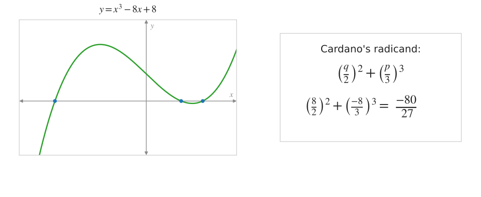
There are now negative numbers under square roots!! If we retrace our steps and work through del Ferro’s method, the problem arises because the disguised quadratic in \(y^{3}\) has negative square roots, and this carries through to the solution of our cubic.

This is the kind of difficulty Cardano encountered: the cubic has a real solution of \(2\) (and two other solutions), but the method brings us to these weird negative roots.

To understand why and how this happens, we must understand the nature of the roots of the cubic. This section will focus on the roots of depressed cubics, but many of the same concepts apply to general cubic equations.

A cubic with real coefficients always has at least one real root, but it may have one, two, or three distinct real roots. As with the quadratics from Chapter 1, a discriminant tells us which case occurs. Figure 2.13 shows the possibilities using the quantity under Cardano's square root, called D; the standard cubic discriminant uses the opposite sign.

Two related discriminants for \(x^{3} + px + q = 0\): \[\Delta = - 4p^{3} - 27q^{2} = - 108D,\quad\quad D = \frac{q^{2}}{4} + \frac{p^{3}}{27}.\] Here \(D\) is Cardano’s square-root radicand; the usual polynomial discriminant is \(\Delta\).
For a cubic with real coefficients: \(\Delta > 0\): three distinct real roots. \(\Delta = 0\): a double and a simple real root, or one triple root. \(\Delta < 0\): one real root and a pair of nonreal complex conjugate roots.

Figure 2.13

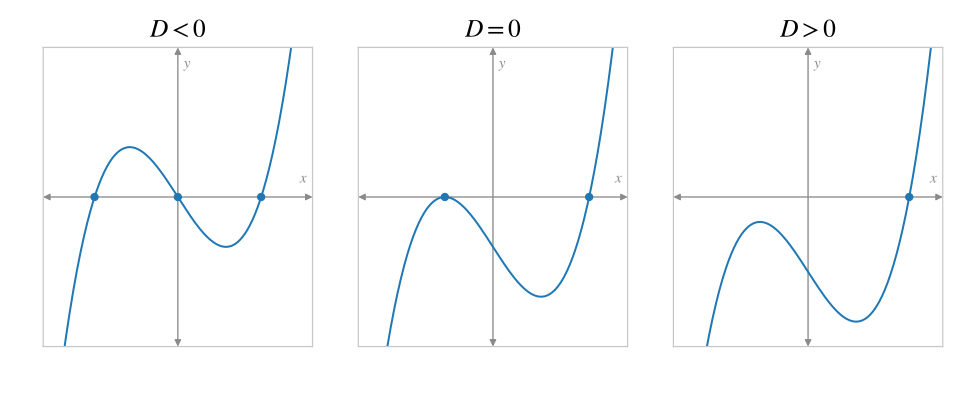
The two discriminant quantities have opposite signs. So when the usual discriminant predicts three distinct real roots, Cardano's radicand is negative. That is exactly why a problem with three real answers can require complex intermediate values. We will return to those strange square roots in Chapter 7.

The Plastic Ratio

Definition

Just as the golden ratio and metallic means arose from quadratic equations, even more magical numbers come from related cubic equations. One of them is known as the plastic ratio, and it comes from a problem similar to the one for the golden ratio.¹³ It arises from a problem involving dividing a line up into three pieces this time, called \(a\), \(b\) and \(c\). The ratio of \(b\) to \(c\), also expressed as \(\frac{b}{c}\), I will call \(\rho\). Therefore

\[b = \rho c\]

We want to scale \(b\) up by the same factor, \(\rho\), to get \(a\), so

\[\frac{a}{b} = \frac{b}{c} = \rho\]

Furthermore, \(a = \rho b\). And, because of the previous relation,

\[a = \rho^{2}c\]

As a second condition, we want the ratio of \(b + c\) to \(a\) to be the same as the above ratios, so

\[\frac{b + c}{a} = \frac{a}{b} = \frac{b}{c}\]

Figure 2.14

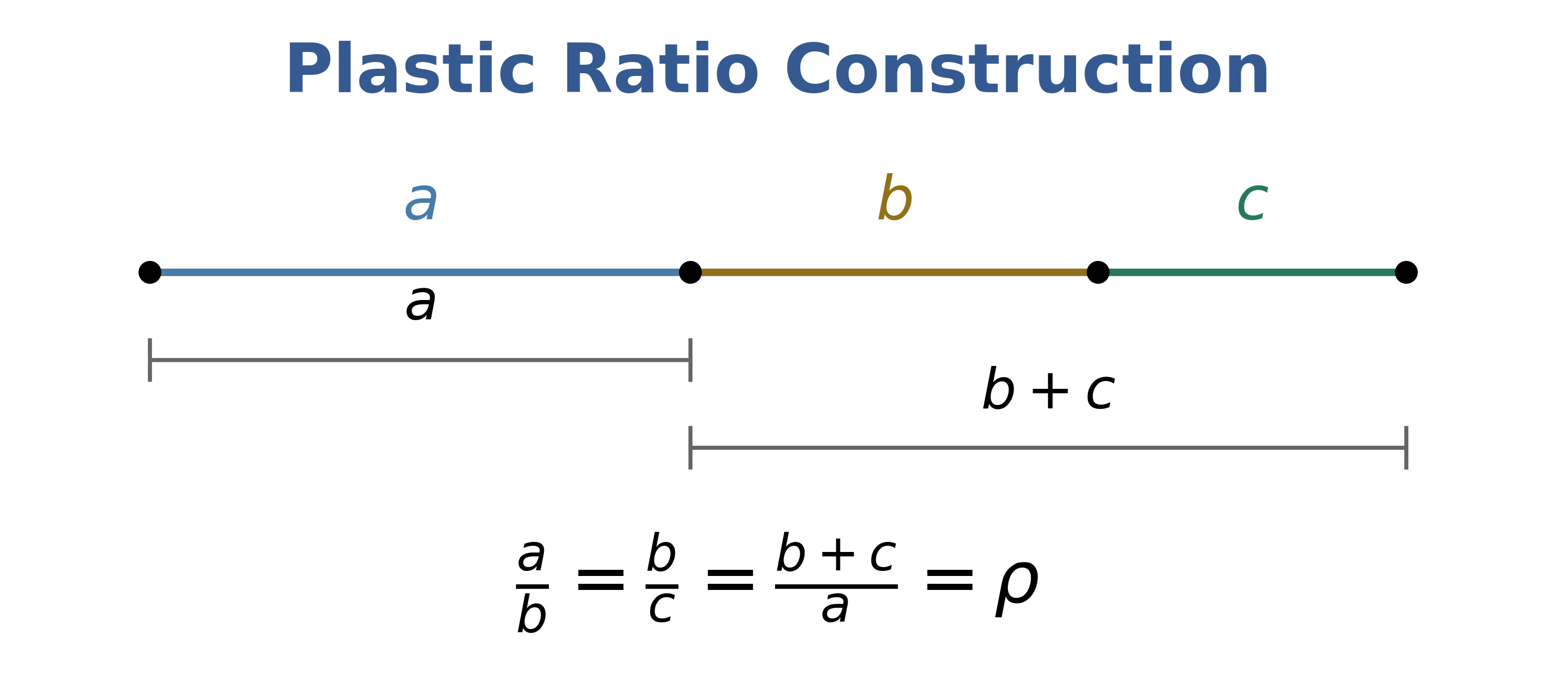
We can assume \(c = 1\), so \(b = \rho\), and \(a = \rho^{2}\).

Because of the last fraction, we get the equation

\[\rho = \frac{\rho + 1}{\rho^{2}}\]

After multiplying through by \(\rho^{2}\), we obtain the cubic equation

\[\boxed{\rho^{3} = \rho + 1}\]

After moving the constants to the left side,

\[\rho^{3} - \rho - 1 = 0\]

We can solve by the depressed cubic formula:

\[\rho = \sqrt[3]{\frac{1}{2} + \sqrt{\left( \frac{1}{2} \right)^{2} + \left( - \frac{1}{3} \right)^{3}}} + \sqrt[3]{\frac{1}{2} - \sqrt{\left( \frac{1}{2} \right)^{2} + \left( - \frac{1}{3} \right)^{3}}}\]

After simplifying, we find

\[\rho = \sqrt[3]{\frac{1}{2} + \frac{\sqrt{69}}{18}} + \sqrt[3]{\frac{1}{2} - \frac{\sqrt{69}}{18}} \approx 1.325\]

This is our plastic ratio!

Exponent Relations

Similar to the golden ratio, higher powers of the plastic ratio can be expressed in terms of lower powers. For example, \(\rho^{4}\) can be written as \(\rho*\rho^{3}\), and we can use the fact that \(\rho^{3} = \rho + 1\) to rewrite our expression as

\[\rho(\rho + 1) = \rho^{2} + \rho = \rho^{4}\]

In general, for any integer power of \(\rho\), we can rewrite it in terms of lower powers like so,

\[\rho^{n} = \rho^{n - 2} + \rho^{n - 3}\]

We can even continue to expand the lower powers into even lower ones.

Since \(\rho^{n - 2} = \rho^{n - 4} + \rho^{n - 5}\), \(\rho^{n} = \rho^{n - 3} + \rho^{n - 4} + \rho^{n - 5}\), by substituting in for \(\rho^{n - 2}\). You could continue coming up with similar identities to infinity.

The Plastic Rectangle

Also, like the golden ratio, the plastic ratio has interesting properties in a rectangle.

A plastic rectangle has the long side of \(\rho\) and a short side of \(1\).

Now, instead of removing a square, we remove a similar rectangle, with the same proportions. The long side is \(1\), and the short side is \(\frac{1}{\rho}\).

Now, on the other side of the rectangle, we remove a square from the top, with side lengths of \(\rho - \frac{1}{\rho}\). In a plastic rectangle, the remaining rectangle on the bottom right is also a similar rectangle, with the same proportions!

Figure 2.15

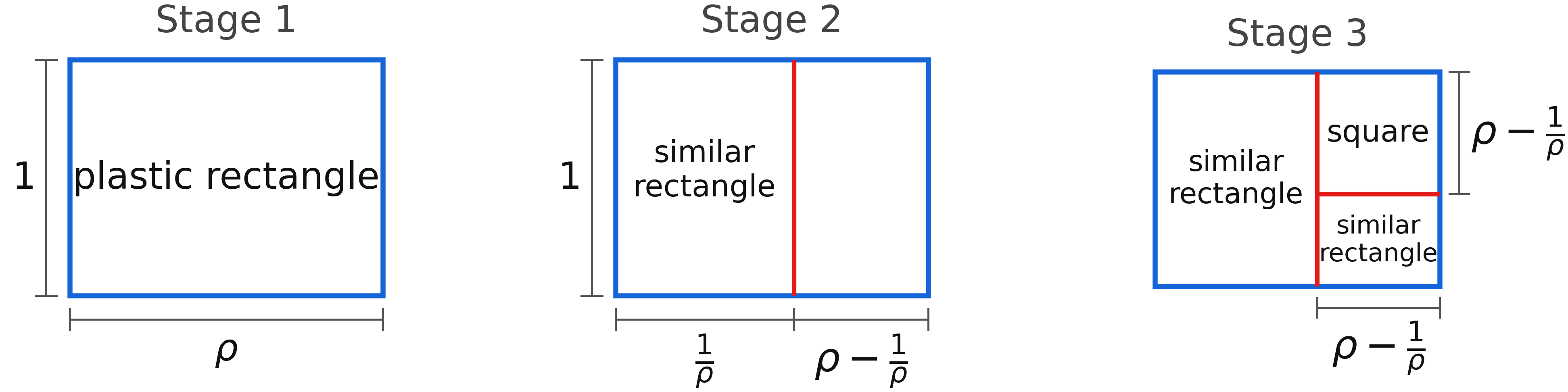
We can easily prove this by looking at opposite sides of the rectangle.

The width of the bottom right rectangle is \(\left( \rho - \frac{1}{\rho} \right) \div \rho = 1 - \frac{1}{\rho^{2}}\)

Because the rectangles are similar, the length is \(\rho\) times the width. Now, the left side of the rectangle is \(1\), and the right side therefore must add to \(1\).

So we get the equation \(1 = \rho - \frac{1}{\rho} + 1 - \frac{1}{\rho^{2}}\). Subtracting \(1\) from both sides, we get \(0 = \rho - \frac{1}{\rho} - \frac{1}{\rho^{2}}\). After multiplying through by \(\rho^{2}\), we get the familiar equation \(\rho^{3} - \rho - 1 = 0\).

Other Geometry

\(\rho\) can also be found in another geometric problem. How can you divide up a square into three similar rectangles, rectangles with the same ratio of short to long sides?

The obvious solution is just to divide up the square into three of the same rectangle, all with aspect ratio \(3:1\).

Another solution comes from using one rectangle to take up \(\frac{2}{3}\) of the square (with aspect ratio \(3:2\)) and using two smaller copies in the remaining third.

The third and last solution, with rectangles of all different sizes (but similar), has rectangles with aspect ratio \(\rho^{2}:1\).

Figure 2.16

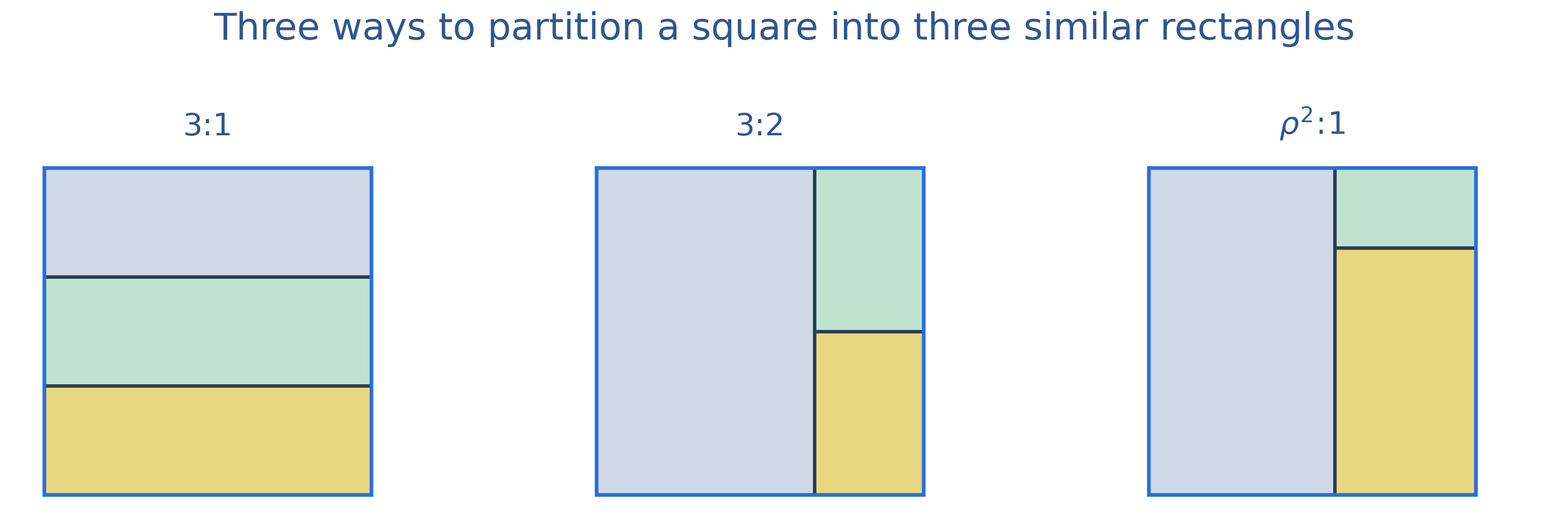
It has been proven that the above solutions are the only ways to divide a square up into three similar rectangles.¹⁴

The Van der Laan Sequence

Just as the golden ratio was related to the Fibonacci numbers, the plastic ratio is related to a similar sequence, called the Van der Laan sequence. It is sometimes also referred to as the Padovan sequence.¹⁵

The Van der Laan sequence is very similar to the Fibonacci sequence, and it starts with the values 1, 1, 1. To generate the next value, you add the second previous number to the third previous number. The sequence goes 1, 1, 1, 2, 2, 3, 4, 5, 7, 9, 12, 16, 21, 28…

Figure 2.17

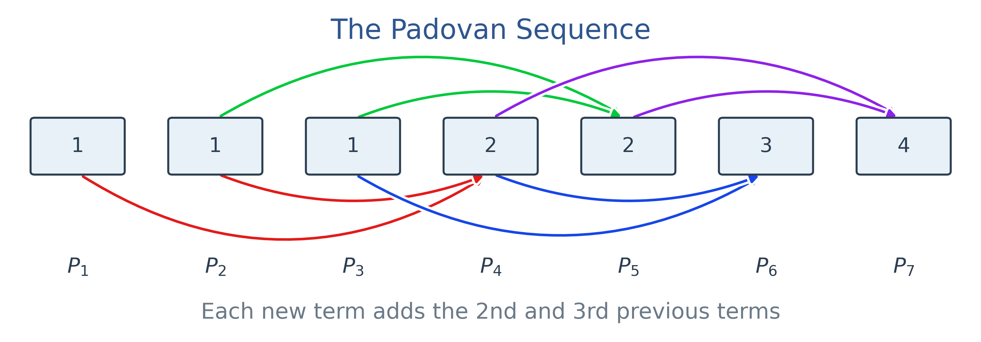
The general expression of the nth term is

\[\boxed{V_{n} = V_{n - 2} + V_{n - 3}}\]

The ratios of successive terms in the sequence approach \(\rho\). After expanding, we can show that the Van der Laan sequence also follows

\[V_{n} = V_{n - 1} + V_{n - 5}\]

Notice the similarities between these relations and our previously derived identities involving \(\rho\). The power of \(\rho\) is replaced with the terms’ index in the sequence. This is not a coincidence, because the ratios of successive terms in this sequence approach \(\rho\).

The Van der Laan sequence can be visualized by equilateral triangles, like how the Fibonacci sequence can be visualized with squares and rectangles.¹⁶

First, place three equilateral triangles with side lengths of \(1\) next to each other.

Next, draw another two equilateral triangle next to the starting structure, with side lengths of \(2\).

Then, draw an equilateral triangle with side length 3 next to a 2 triangle and a 1 triangle as shown.

Figure 2.18

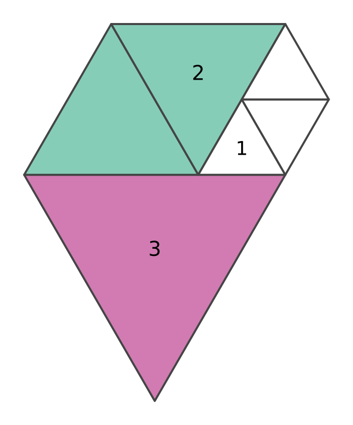
This shows the relation \(V_{n} = V_{n - 1} + V_{n - 5}\) geometrically (since the side length of the previous triangle is added to the fifth previous one).

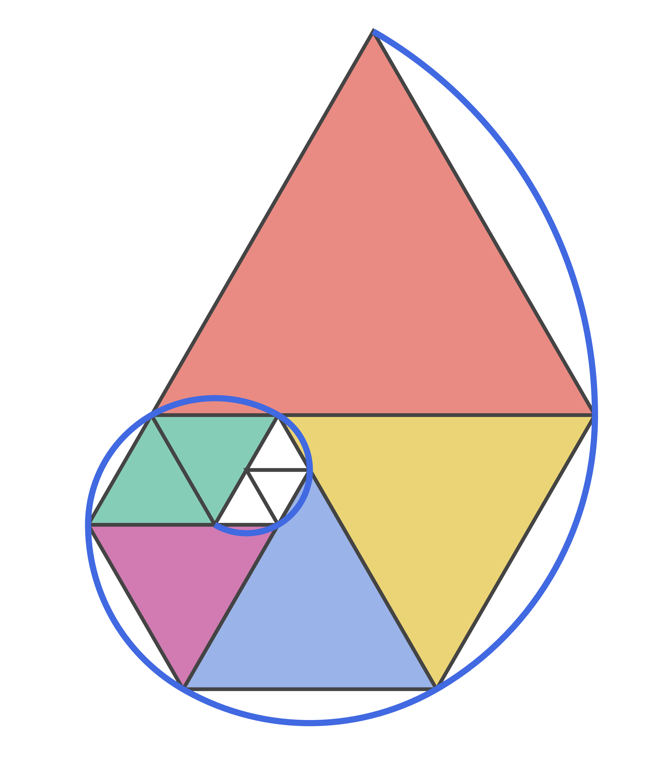
We can also do this construction in reverse, starting with a large equilateral triangle and adding smaller ones on the side. To do this, we scale down each successive triangle by \(1/\rho\), which is approximately \(3/4\).

We can decorate this with parts of a circle on the outsides of the triangles, forming a plastic spiral:

Figure 2.19

The Supergolden Ratio

Definition

There is another number related to both the golden ratio and cubic equations, and it is called the supergolden ratio.¹⁷ It also arises from a problem involving dividing a segment into three pieces, but in a different way.

Figure 2.20

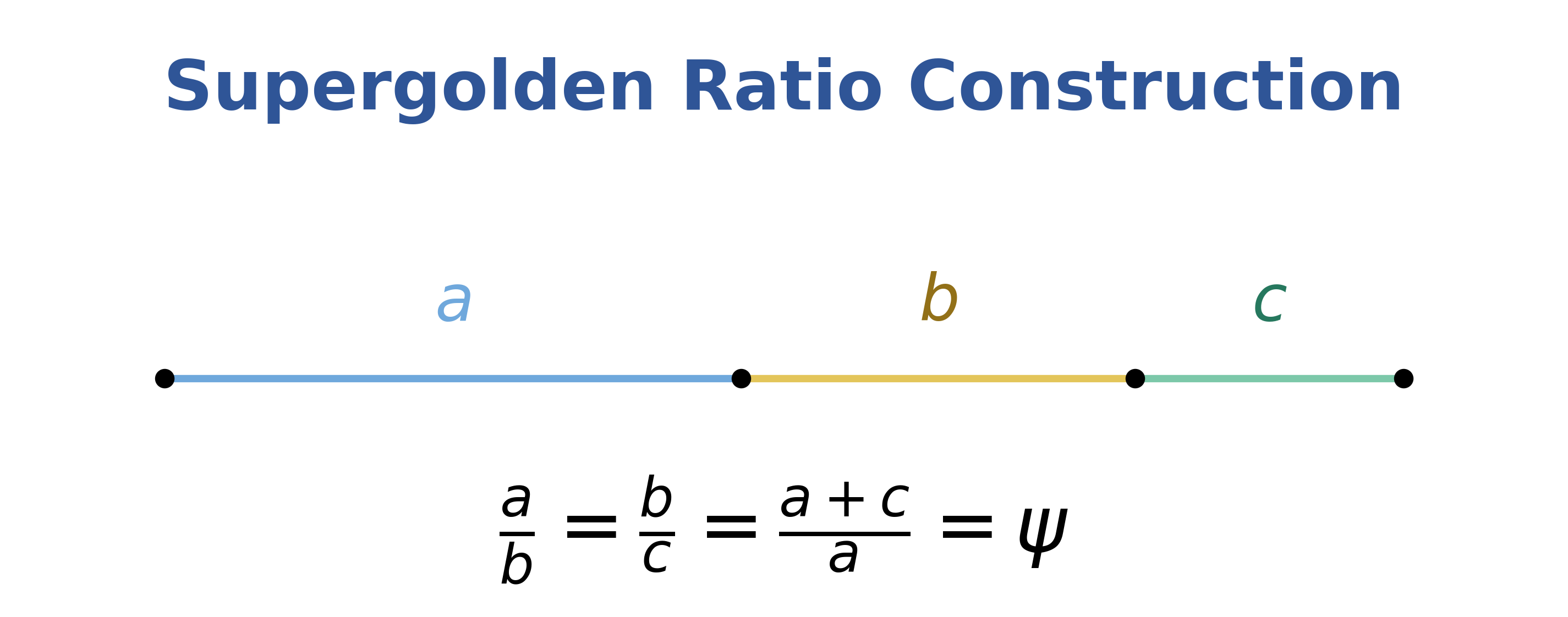
We have a line segment, and we divide it up into three pieces, \(a\), \(b\), and \(c\).

We want the ratios \(a:b\) and \(b:c\) to be the same (multiplying by the same number), so

\[\frac{a}{b} = \frac{b}{c}\]

This ratio is denoted by \(\psi\). Therefore \(a = \psi b\), and \(b = \psi c\).

Furthermore, \(a = \psi^{2}c\).

This time, the defining ratio is the segment \(a + c:a\).

We can set up an equation,

\[\psi = \frac{a + c}{a}\]

We now substitute \(a = \psi^{2}*c\) to eliminate \(a\),

\[\psi = \frac{\psi^{2}c + c}{\psi^{2}c}\]

Now we can factor out \(c\) in the fraction and cancel it:

\[\psi = \frac{\left( \psi^{2} + 1 \right)c}{\psi^{2}c}\]

\[\psi = \frac{\psi^{2} + 1}{\psi^{2}}\]

After multiplying by \(\psi^{2}\), we get a cubic equation for \(\psi\):

\[\boxed{\psi^{3} = \psi^{2} + 1}\]

This is very similar looking to the plastic ratio, except for the \(\psi^{2}\) term on the right hand side. Applying the general cubic formula would be a bit unwieldy, so it would be wise to depress the cubic first. We rearrange to get all terms on one side: \(\psi^{3} - \psi^{2} - 1 = 0\). Now we can substitute \(\psi = w + \frac{1}{3}\). After collecting like terms, we get the depressed cubic

\[w^{3} - \frac{1}{3}w - \frac{29}{27} = 0\]

Solving by the depressed cubic formula:

\[w = \sqrt[3]{\frac{29}{54} + \sqrt{\left( \frac{29}{54} \right)^{2} + \left( - \frac{1}{9} \right)^{3}}} + \sqrt[3]{\frac{29}{54} - \sqrt{\left( \frac{29}{54} \right)^{2} + \left( - \frac{1}{9} \right)^{3}}}\]

We can simplify after expanding the squares and cubes:

\[w = \sqrt[3]{\frac{29}{54} + \sqrt{\frac{31}{108}}} + \sqrt[3]{\frac{29}{54} - \sqrt{\frac{31}{108}}}\]

Now we can back substitute \(\psi = w + \frac{1}{3}\) to get an expression for \(\psi\):

\[\psi = \sqrt[3]{\frac{29}{54} + \sqrt{\frac{31}{108}}} + \sqrt[3]{\frac{29}{54} - \sqrt{\frac{31}{108}}} + \frac{1}{3}\]

This expression shows that \(\psi \approx 1.466\), which is a more manageable form of the answer.

Properties and Identities

We can come up with some interesting properties and identities by playing with the original equation \(\psi^{3} = \psi^{2} + 1\).

Multiplying both sides by \(\psi^{n - 3}\), where \(n\) is any integer (or more generally any number), we get the formula

\[\psi^{n} = \psi^{n - 1} + \psi^{n - 3}\]

Furthermore, we can decompose \(\psi^{n - 1}\) into lower powers by the above formula and plug back in: \(\psi^{n - 1} = \psi^{n - 2} + \psi^{n - 4}\); therefore

\[\psi^{n} = \psi^{n - 2} + \psi^{n - 3} + \psi^{n - 4}\]

The Supergolden Rectangle

Some interesting properties arise in the supergolden rectangle, a rectangle with a long side of \(\psi\) and a short side of \(1\).

Figure 2.21

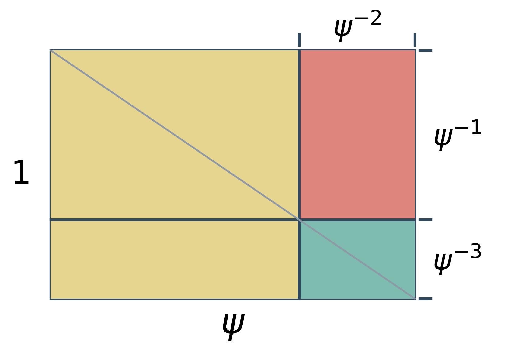
One of the more obvious properties is the length of the diagonal. According to the Pythagorean theorem, a famous theorem in geometry (that was known long before Pythagoras),¹⁸ if we call the two sides of the triangle \(a\) and \(b\), the long side, \(c\), is \(\sqrt{a^{2} + b^{2}}\). Plugging in, we get

\[c = \sqrt{\psi^{2} + 1}\]

But we already know that \(\psi^{2} + 1 = \psi^{3}\), so by substitution

\[c = \sqrt{\psi^{3}}\]

Another property comes again from removing squares from the rectangle. If we remove a square from the left side of the rectangle, the remaining length is \(\psi - 1\).

Rearranging the cubic equation that defines \(\psi\), we find

\[\psi^{3} - \psi^{2} = 1\]

After dividing by \(\psi^{2}\), we find

\[\psi - 1 = \frac{1}{\psi^{2}} = \psi^{- 2}\]

This means that this length is also \(\psi^{- 2}\).

Now, we can draw a rectangle similar to the first in the top right corner, with long side \(\frac{1}{\psi} = \psi^{- 1}\) and short side \(\psi^{- 2}\).

This has the very nice property that the bottom side lines up with where the square intersects the diagonal.

The bottom right rectangle has a long side of \(\psi^{- 2}\), and a short side of \(1 - \psi^{- 1}\). We can rewrite the short side by dividing the defining equation \(\psi^{3} - \psi^{2} = 1\) by \(\psi^{3}\) this time:

\[1 - \psi^{- 1} = \psi^{- 3}\]

So the short side is \(\psi^{- 3}\), and by the same logic the bottom right rectangle is also a similar rectangle!

Extending the line segment to the left, we find yet another similar rectangle in the top left, with long side \(1\) and short side \(\psi^{- 1}\). This gives three similar rectangles inside one larger supergolden rectangle.

The final rectangle, in the bottom left, has dimensions \(1\) by \(\psi^{- 3}\), and thus is not a similar copy, but a rectangle with its own proportions and properties.

The Narayana Sequence

The supergolden ratio’s defining sequence is known as the Narayana sequence, named after the 14th-century mathematician Narayana Pandita, who posed a cow-herd problem that leads to this sequence.

Here is a modern version of the problem: If a cow herd starts with 1 newborn cow at year 1, none of the cows die, and each cow gives birth to another cow once a year from age 3 onwards (so the first calf arrives in year 4), how many cows will there be at year 20?

The number of cows in year \(n\) forms the Narayana sequence.¹⁹

To construct the sequence, we first start with three ones: 1, 1, 1. Now, to get the next element, add the previous number to the third previous number. Or, in mathematical terms:

\[\boxed{N_{m} = N_{m - 1} + N_{m - 3}}\]

This sequence goes 1, 1, 1, 2, 3, 4, 6, 9, 13, 19, 28, 41… Ratios of each term to the term before it approach the supergolden ratio:

\(\frac{N_{m}}{N_{m - 1}} \approx \psi\ \ \ \) ²⁰

Figure 2.22

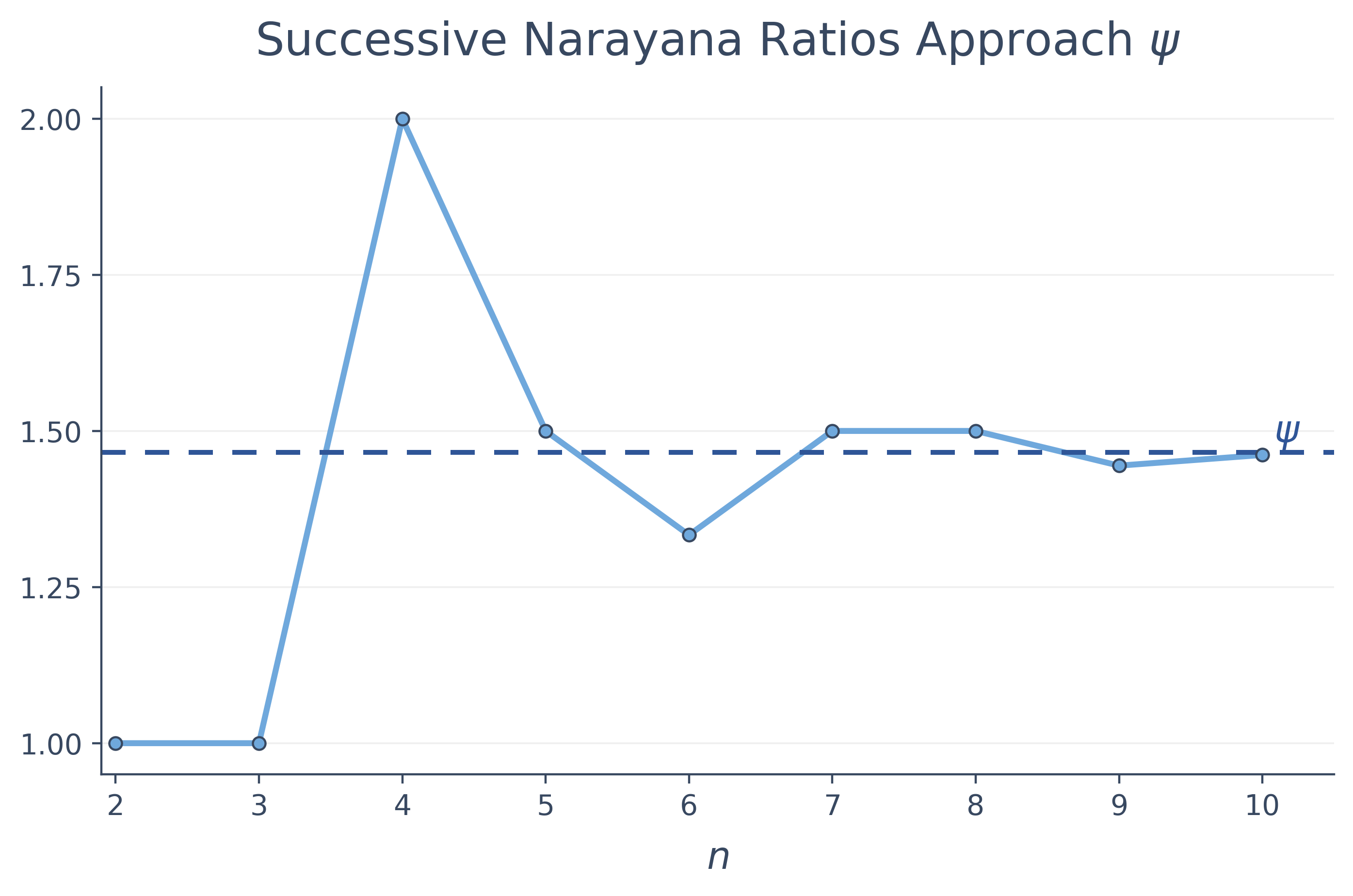
We already know the approximate value of the supergolden ratio: \(\psi \approx 1.4656\). Taking ratios of successive Narayana numbers, we get \(\frac{9}{6} = 1.5\); \(\frac{13}{9} \approx 1.444\); \(\frac{19}{13} \approx 1.4615\).

We are already relatively close to \(\psi\), even though the numbers are less than 20.

We have found cubic equations in some unexpected places, including the plastic and supergolden ratios. But solving a cubic has another use, one that takes us back to Ferrari from the historical section. Remember that he discovered a method for solving quartic equations, and that one of the steps involved solving a cubic. That might seem strange. Why would we need an equation of degree three to solve one of degree four?

We already have a method for finding the roots of cubics, so we can put it to work on the next problem. Let’s see how Ferrari used the cubic to solve the quartic.

← Previous chapter Book contents Next chapter →

Footnotes

1. J. J. O’Connor and E. F. Robertson, “Quadratic, Cubic and Quartic Equations,” MacTutor History of Mathematics Archive, University of St Andrews, accessed October 14, 2026, https://mathshistory.st-andrews.ac.uk/HistTopics/Quadratic_etc_equations/ J. J. O’Connor and E. F. Robertson, “Nine Chapters on the Mathematical Art,” MacTutor History of Mathematics Archive, University of St Andrews, accessed October 14, 2026, https://mathshistory.st-andrews.ac.uk/HistTopics/Nine_chapters/

2. For Khayyam’s conic solutions, see Bijan Vahabzadeh, “Khayyam, Omar xiv. As Mathematician,” Encyclopaedia Iranica, May 7, 2014, updated August 29, 2017, https://www.iranicaonline.org/articles/khayyam-omar/khayyam-omar-xiv-as-mathematician/.

3. J. J. O’Connor and E. F. Robertson, “Scipione del Ferro,” MacTutor History of Mathematics Archive, University of St Andrews, accessed October 14, 2026, https://mathshistory.st-andrews.ac.uk/Biographies/Ferro/

4. J. J. O’Connor and E. F. Robertson, “Tartaglia versus Cardan,” MacTutor History of Mathematics Archive, University of St Andrews, accessed October 14, 2026, https://mathshistory.st-andrews.ac.uk/HistTopics/Tartaglia_v_Cardan/ J. J. O’Connor and E. F. Robertson, “Tartaglia,” MacTutor History of Mathematics Archive, University of St Andrews, accessed October 14, 2026, https://mathshistory.st-andrews.ac.uk/Biographies/Tartaglia/

5. O’Connor and Robertson, “Tartaglia versus Cardan.” J. J. O’Connor and E. F. Robertson, “Girolamo Cardano,” MacTutor History of Mathematics Archive, University of St Andrews, accessed October 14, 2026, https://mathshistory.st-andrews.ac.uk/Biographies/Cardan/

6. William B. Branson, “Solving the Cubic with Cardano,” Convergence (September 2013), https://doi.org/10.4169/convergence20131001.

7. J. J. O’Connor and E. F. Robertson, “Lodovico Ferrari,” MacTutor History of Mathematics Archive, University of St Andrews, accessed October 14, 2026, https://mathshistory.st-andrews.ac.uk/Biographies/Ferrari/

8. O’Connor and Robertson, “Scipione del Ferro.” O’Connor and Robertson, “Girolamo Cardano.”

9. Tony Rothman, “Cardano v Tartaglia: The Great Feud Goes Supernatural,” author preprint, 2013, 7–8, 13–14, https://arxiv.org/pdf/1308.2181. O’Connor and Robertson, “Tartaglia.” The exact course of the debate is not recorded, and accounts of the dispute reflect the participants’ interests.

10. O’Connor and Robertson, “Quadratic, Cubic and Quartic Equations.” O’Connor and Robertson, “Tartaglia versus Cardan.”

11. For Cardano’s geometric treatment and a modern presentation, see Branson, “Solving the Cubic with Cardano.”

12. For a related approach by completing powers, see Hua-Lin Huang, Shengyuan Ruan, Xiaodan Xu, and Yu Ye, “Solving Cubic Equations by Completing the Cube and Higher Degree Equations by Completing Powers,” authors’ preprint, version 3, sec. 3, https://arxiv.org/html/2301.07375v3. This is a related method, not a claim that the exact derivation presented here is the same.

13. Vera W. de Spinadel and Antonia Redondo Buitrago, “Towards van der Laan’s Plastic Number in the Plane,” Journal for Geometry and Graphics 13, no. 2 (2009): 163–175, https://www.heldermann-verlag.de/jgg/jgg13/j13h2spin.pdf.

14. Byung-Kyu Chun, Andy Liu, and Daniel van Vliet, “Dissecting Squares into Similar Rectangles,” Crux Mathematicorum 22 (1996): 241–248, https://www.cms.math.ca/wp-content/uploads/crux-pdfs/CRUXv22n6.pdf. de Spinadel and Redondo Buitrago, “Towards van der Laan’s Plastic Number in the Plane.”

15. de Spinadel and Redondo Buitrago, “Towards van der Laan’s Plastic Number in the Plane.”

16. de Spinadel and Redondo Buitrago, “Towards van der Laan’s Plastic Number in the Plane.” See 165–166, especially figure 5.

17. The On-Line Encyclopedia of Integer Sequences, “A092526,” accessed October 14, 2026, https://oeis.org/A092526.

18. J. J. O’Connor and E. F. Robertson, “Pythagoras’s Theorem in Babylonian Mathematics,” MacTutor History of Mathematics Archive, University of St Andrews, accessed October 14, 2026, https://mathshistory.st-andrews.ac.uk/HistTopics/Babylonian_Pythagoras/

19. Prasad Jawalgekar, D. G. Sooryanarayan, and K. Ramasubramanian, “Gaṇitakaumudī of Nārāyaṇa Paṇḍita: A Gem among the Pāṭīgaṇita Texts in Indian Mathematics,” Bhāvanā 7, no. 1 (January 2023), “Progressions,” verse 16, https://bhavana.org.in/ga%E1%B9%87itakaumudi-of-naraya%E1%B9%87a-pa%E1%B9%87%E1%B8%8Dita/. The original problem begins with a cow already reproducing; the text here explicitly uses a modern newborn-at-year-1 convention.

20. OEIS, “A092526.”