Chapter 6: Hyperbolic Trigonometry

There is an amazing extension of trigonometry based on a curve known as a hyperbola called hyperbolic trigonometry. However, there are some prerequisites to gain an understanding of hyperbolic trigonometry. The first is expressing the trig functions in terms of areas, and the second is the fundamental mathematical constant \(e\), introduced in Chapter 5½.

Trigonometry Defined With Areas

In Chapters 4 and 5, we have looked at the trigonometric functions in terms of angles, where you input an angle and get a certain length related to the unit circle. Because of the properties of the unit circle, we can also express inputs to the trigonometric functions in terms of areas.

Recall that the full distance around a circle is \(\tau\) times the radius, or \(2\pi\) times the radius. Because \(\tau\) radians makes up a full circle, \(\frac{1}{4}\) of a circle is \(\frac{\tau}{4}\) radians. The area of the unit circle is \(\pi\) square units, so it follows that the area of \(\frac{1}{4}\) of a circle is \(\frac{\pi}{4}\) square units.

Figure 6.1

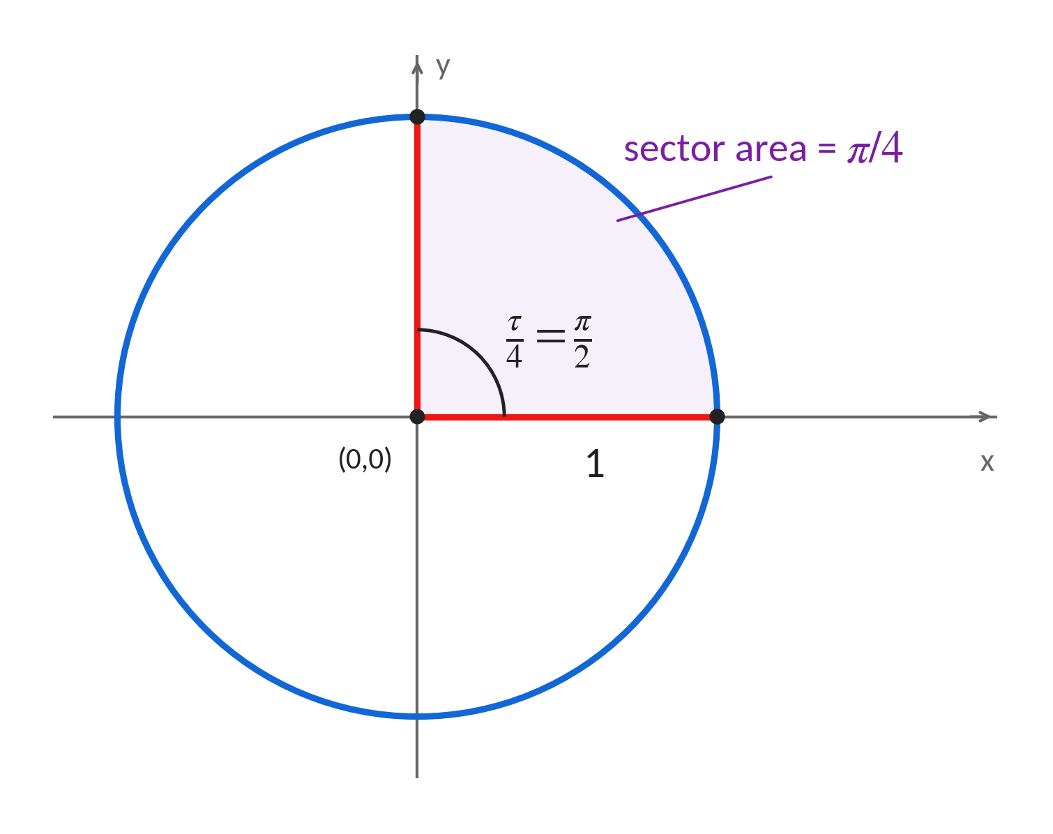
Because \(\tau\) is simply double \(\pi\), this means that for an angle measured counterclockwise from 0 to \(\tau\) on the unit circle, the area swept out by that angle is half of the angle itself (in radians). Now, we can express the trigonometric functions as functions of areas of circular sectors. If \(a\) is the area of the circular sector, \(\frac{\theta}{2} = a\), so \(\theta = 2a\). So, I can draw a point on the unit circle and measure the area between the x-axis and the point, like this:

Figure 6.2

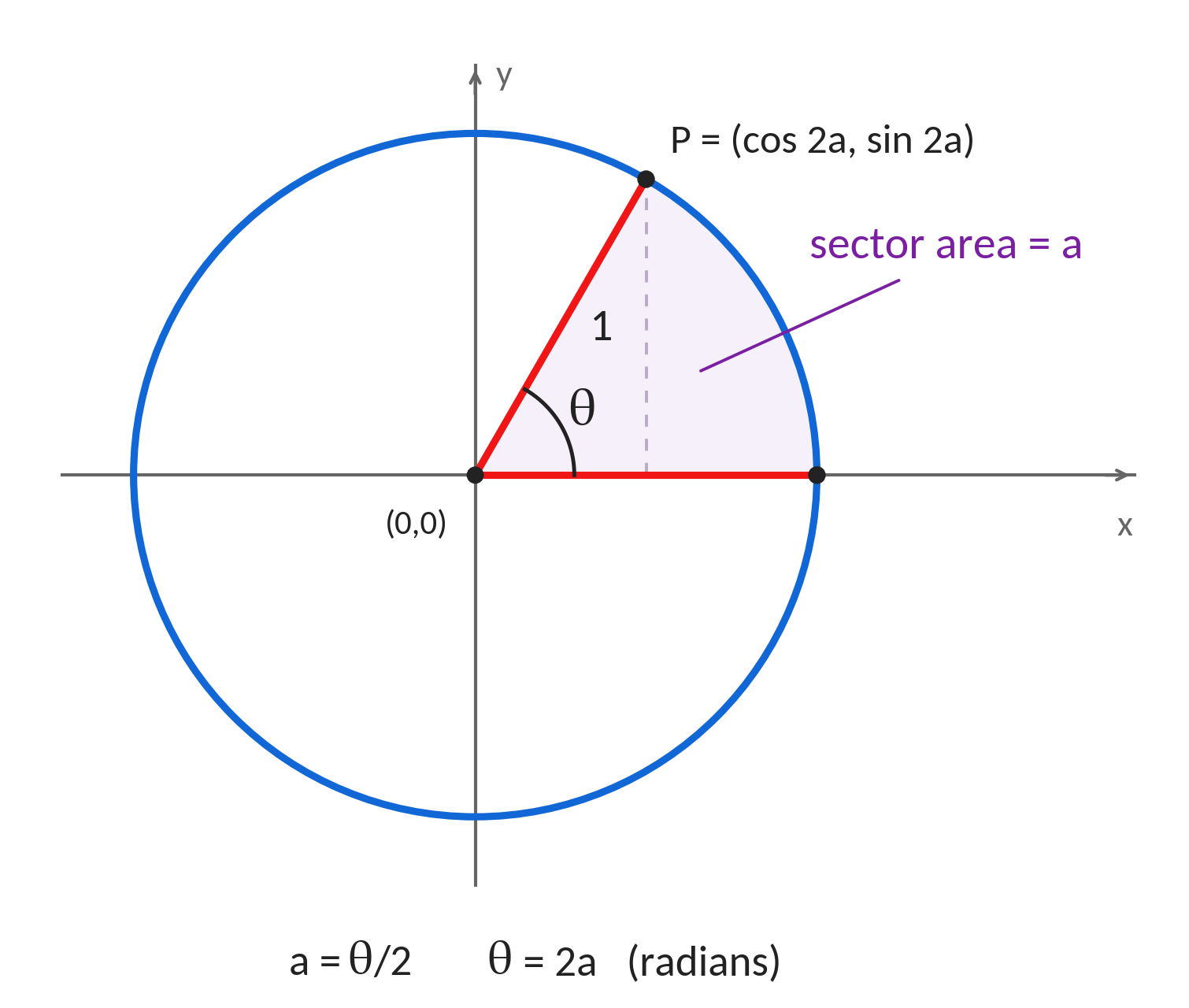
The x-coordinate of the point is \(\cos(2a)\) by substituting for \(\theta\). Similarly, the y-coordinate is \(sin(2a)\). Soon we will see this idea is applicable to a different curve, a hyperbola.

Defining Hyperbolic Functions

Now that we have an understanding of the number \(e\) and how to represent inputs to the trigonometric functions as areas, we can fully investigate hyperbolic trigonometry. Recall how the unit circle was defined by the equation

\[x^{2} + y^{2} = 1\]

In contrast, the unit hyperbola is defined by the equation

\[x^{2} - y^{2} = 1\]

and looks like this:

Figure 6.3

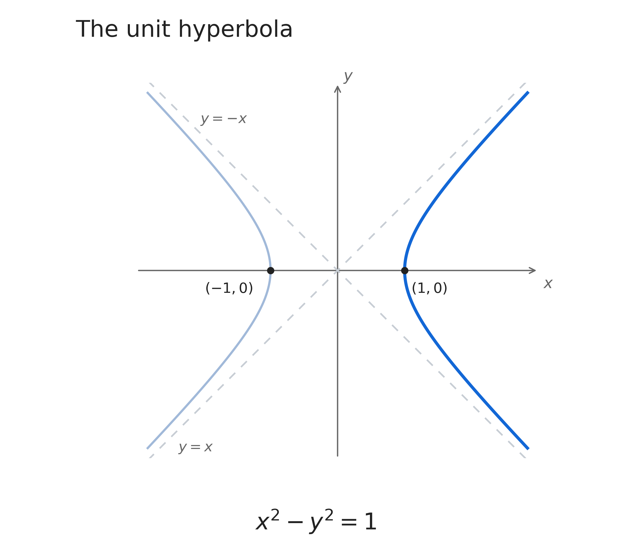
Similarly to how we used areas of circular sectors above, we can now draw a line from the origin to a point on the right branch of the hyperbola and define the area of a “hyperbolic sector” as the shaded portion in the picture:

Figure 6.4

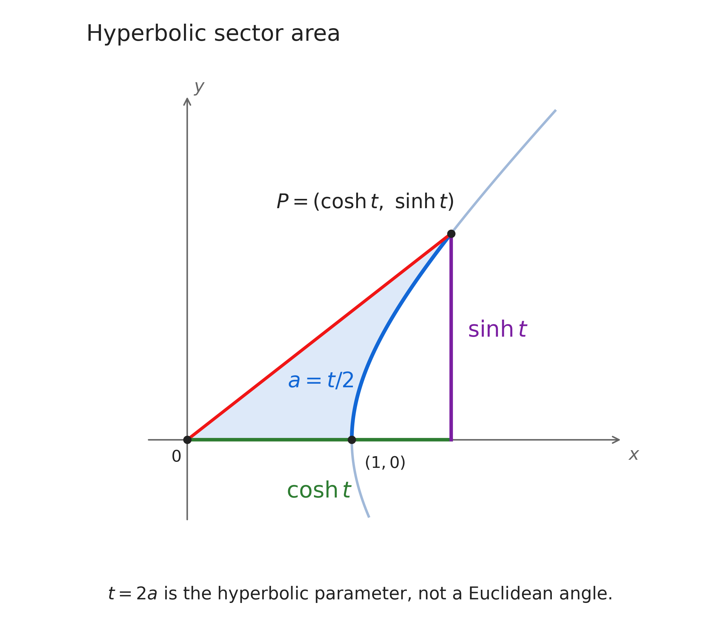
On the circle, you could find the x and y coordinates by plugging in twice the area to the regular trig functions. So, it makes sense that we can define some sort of hyperbolic trig function that takes in twice the area and gives back the x or y coordinates.

Hyperbolic cosine, denoted by cosh, should satisfy \(\cosh(2a) = x\), where \(a\) is the area of the sector.

Hyperbolic sine, denoted by sinh, should satisfy \(\sinh(2a) = y\).

Gerardus Mercator’s famous map projection involved mathematics that we can now express using hyperbolic functions, although Mercator did not use the functions themselves. The hyperbolic functions were introduced in the 18th century by Vincenzo Riccati and developed further by Johann Heinrich Lambert. This is where modern notation for these functions arose, and much of the content in later chapters involving these functions came from that era.¹

There is only one slight problem with the area definition. What does negative area mean? A natural way to define negative area is that the area of a sector above the x-axis is positive (which we have been looking at up to now) and the area below the x-axis is negative.

Figure 6.5

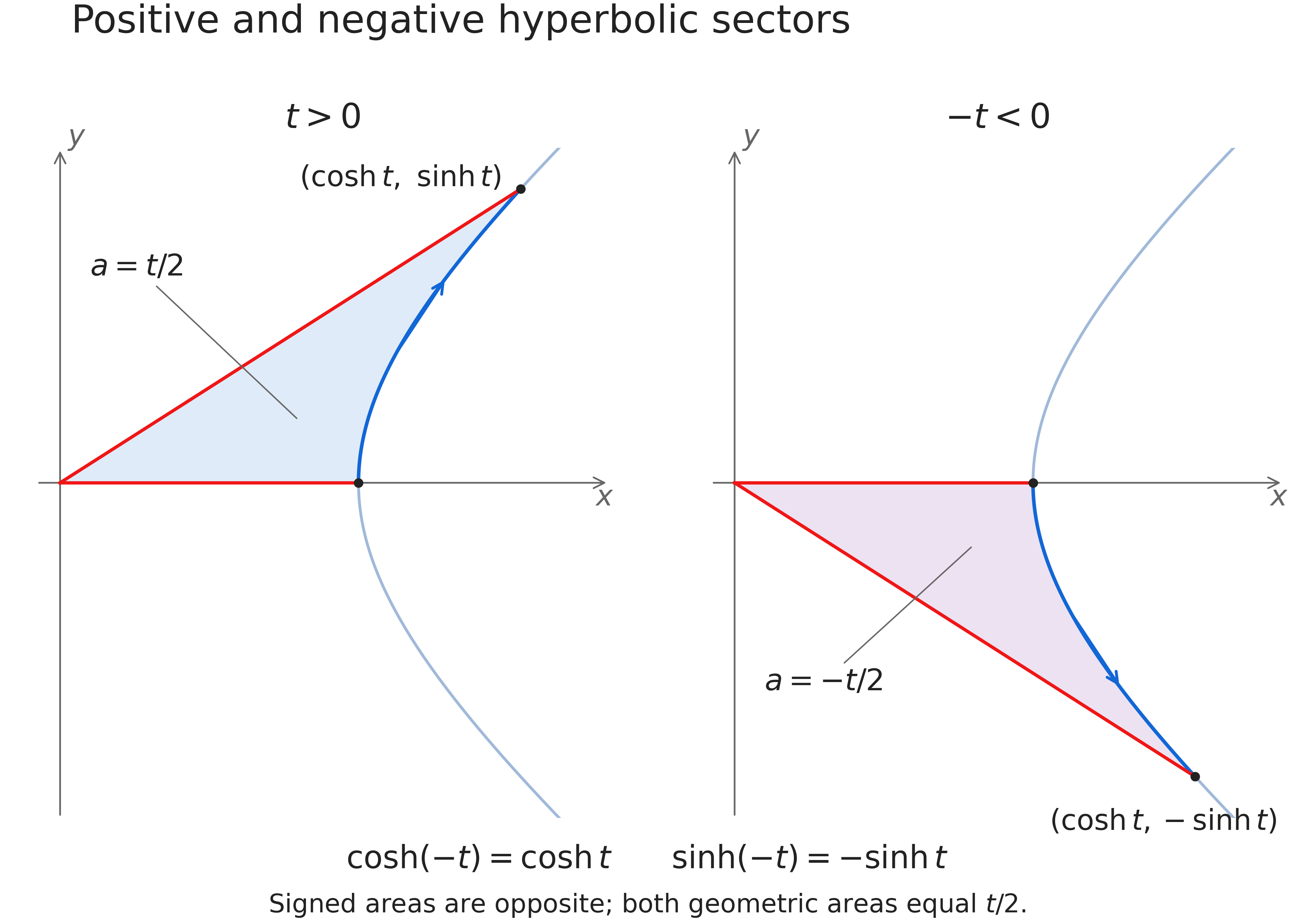
Because the x-coordinate stays the same when the area is negative or positive,

\[\cosh( - a) = \cosh(a)\]

In addition, with negative area the y-coordinate becomes negative, so

\[\sinh( - a) = - sinh(a)\]

The area definition tells us which coordinates cosh and sinh give back, but it does not yet give us formulas for calculating them.

Exponential Forms of Hyperbolic Functions

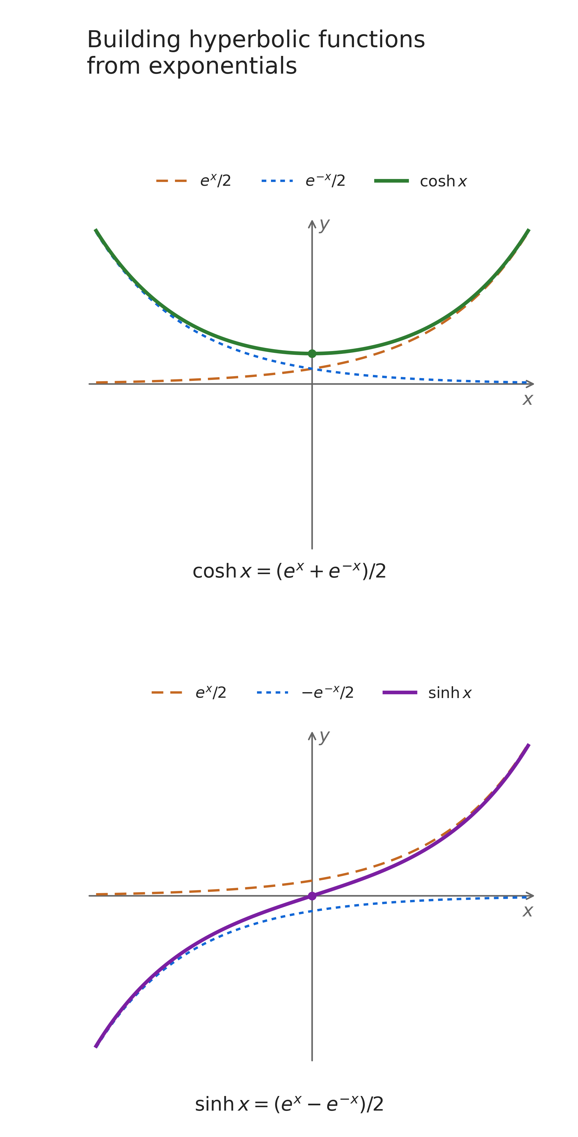
We can also express these functions in terms of \(e\). For any real number \(t\),

\[\boxed{\cosh t = \frac{e^{t} + e^{- t}}{2},\quad\quad\sinh t = \frac{e^{t} - e^{- t}}{2}.}\]

To see how these expressions fit the hyperbola, recall that its coordinates must satisfy

\[x^{2} - y^{2} = 1\]

Squaring the two expressions gives the same exponential terms, so subtracting cancels them:

\[\cosh^{2}t - \sinh^{2}t = \frac{\left( e^{t} + e^{- t} \right)^{2} - \left( e^{t} - e^{- t} \right)^{2}}{4}\]

\[= \frac{\left( e^{2t} + 2 + e^{- 2t} \right) - \left( e^{2t} - 2 + e^{- 2t} \right)}{4} = 1\]

The exponential terms are gone, leaving 1, as required.

When \(t\) is zero, both exponentials are 1, so

\[\cosh\ 0 = 1,\quad\quad\sinh\ 0 = 0\]

This gives the point \((1,0)\), where the sector has zero area. Now, replacing \(t\) with \(- t\) switches \(e^{t}\) and \(e^{- t}\). Because adding them in either order gives the same result, cosh stays the same. Subtracting them in the opposite order changes the sign, so

\[\boxed{\cosh( - t) = cosh\ t,\quad\quad\sinh( - t) = - sinh\ t.}\]

This agrees with what happened to the coordinates when we made the area negative. It does not yet prove that \(t\) is twice the signed sector area; that requires a separate argument.

Figure 6.6

From the functions sinh and cosh, we can find all of the other hyperbolic functions. Recall that \(\tan(x) = \frac{\sin(x)}{\cos(x)}\), so our hyperbolic tangent function is

\[\tanh(x) = \frac{\sinh(x)}{\cosh(x)}\]

Hyperbolic tangent can also be thought of as the slope of the line from the origin to the hyperbola when its input is twice the signed area of the hyperbolic sector.

We can find our other analogous trig functions from related identities, so

\[\begin{aligned}\operatorname{sech}(x) &= \frac{1}{\cosh(x)} \\[0.9em] \operatorname{csch}(x) &= \frac{1}{\sinh(x)} \\[0.9em] \operatorname{coth}(x) &= \frac{\cosh(x)}{\sinh(x)}\end{aligned}\]

Because the hyperbola is defined by the equation \(x^{2} - y^{2} = 1\), the two basic hyperbolic functions obey the similar identity of

\[\boxed{\cosh^{2}(a) - \sinh^{2}(a) = 1}\]

This identity looks very similar to circular trigonometry, except that hyperbolic sine is subtracted instead of added.

Connections to Circular Trigonometry

In fact, there is a far more general rule known as Osborn’s rule that relates the regular trig functions with the hyperbolic versions.² For the standard identities used here, it provides a shortcut: replace regular trig functions with their hyperbolic versions and change the sign for each pair of hyperbolic sine factors, such as two \(\sinh(x)\) factors.

We can already see how this applies to the identity proved above: because

\[\sinh^{2}(x) = \sinh(x)\sinh(x)\]

we change the sign from positive to negative.

For a second example, let’s translate the identity

\[\tan^{2}(x) + 1 = \sec^{2}(x)\]

into a related hyperbolic identity. We must remember that

\[\tanh(x) = \frac{\sinh(x)}{cosh(x)}\]

So, when \(\tanh(x)\) is squared it contains what is called an implied product of two sinhs. This product is “hidden” inside the \(\tanh(x)\) function, but still counts. So our new hyperbolic identity, after the sign is changed, is

\[{1 - \tanh^{2}(x) = sech}^{2}(x)\]

For the addition, double-angle and triple-angle identities used here, the same sign bookkeeping works after products are expanded or denominators are cleared. Higher powers require counting every pair: a fourth power contains two pairs, so its sign changes twice. The shortcut is not a rule for arbitrary expressions or inequalities.

Circular and hyperbolic identities

Circular	Hyperbolic
Fundamental \[\cos^{2}u + \sin^{2}u = 1\]	Fundamental \[\cosh^{2}u - \sinh^{2}u = 1\]
Tangent square \[1 + \tan^{2}u = \sec^{2}u\]	Tangent square \[1 - \tanh^{2}u = {sech}^{2}u\]
Cotangent square \[\cot^{2}u + 1 = \csc^{2}u\]	Cotangent square \[\coth^{2}u - 1 = {csch}^{2}u\]
Sine sum / difference \[\sin(u \pm v) = \sin u\ \cos v \pm cosu\ \sin v\]	Sine sum / difference \[\sinh(u \pm v) = \sinh u\ \cosh v \pm coshu\ \sinh v\]
Cosine sum / difference \[\cos(u \pm v) = \cos u\ \cos v \mp sinu\ \sin v\]	Cosine sum / difference \[\cosh(u \pm v) = \cosh u\ \cosh v \pm sinhu\ \sinh v\]
Tangent sum / difference \[\tan(u \pm v) = \frac{\tan u \pm tanv}{1 \mp tanu\ \tan v}\]	Tangent sum / difference \[\tanh(u \pm v) = \frac{\tanh u \pm tanhv}{1 \pm tanhu\ \tanh v}\]
Sine double angle \[\sin(2u) = 2\sin u\cos u\]	Sine double angle \[\sinh(2u) = 2\sinh u\ \cosh u\]
Cosine double angle \[\cos(2u) = \cos^{2}u - \sin^{2}u\]	Cosine double angle \[\cosh(2u) = \cosh^{2}u + \sinh^{2}u\]
Tangent double angle \[\tan(2u) = \frac{2\tan u}{1 - \tan^{2}u}\]	Tangent double angle \[\tanh(2u) = \frac{2\tanh u}{1 + \tanh^{2}u}\]
Sine triple angle \[\sin(3u) = 3\sin u - 4\sin^{3}u\]	Sine triple angle \[\sinh(3u) = 3\sinh u + 4\sinh^{3}u\]
Cosine triple angle \[\cos(3u) = 4\cos^{3}u - 3\cos u\]	Cosine triple angle \[\cosh(3u) = 4\cosh^{3}u - 3\cosh u\]
Tangent triple angle \[\tan(3u) = \frac{3\tan u - \tan^{3}u}{1 - 3\tan^{2}u}\]	Tangent triple angle \[\tanh(3u) = \frac{3\tanh u + \tanh^{3}u}{1 + 3\tanh^{2}u}\]
Cosine power reduction \[\cos^{2}u = \frac{1 + \cos(2u)}{2}\]	Cosine power reduction \[\cosh^{2}u = \frac{1 + \cosh(2u)}{2}\]
Sine power reduction \[\sin^{2}u = \frac{1 - \cos(2u)}{2}\]	Sine power reduction \[\sinh^{2}u = \frac{\cosh(2u) - 1}{2}\]

Graphs of Hyperbolic Functions

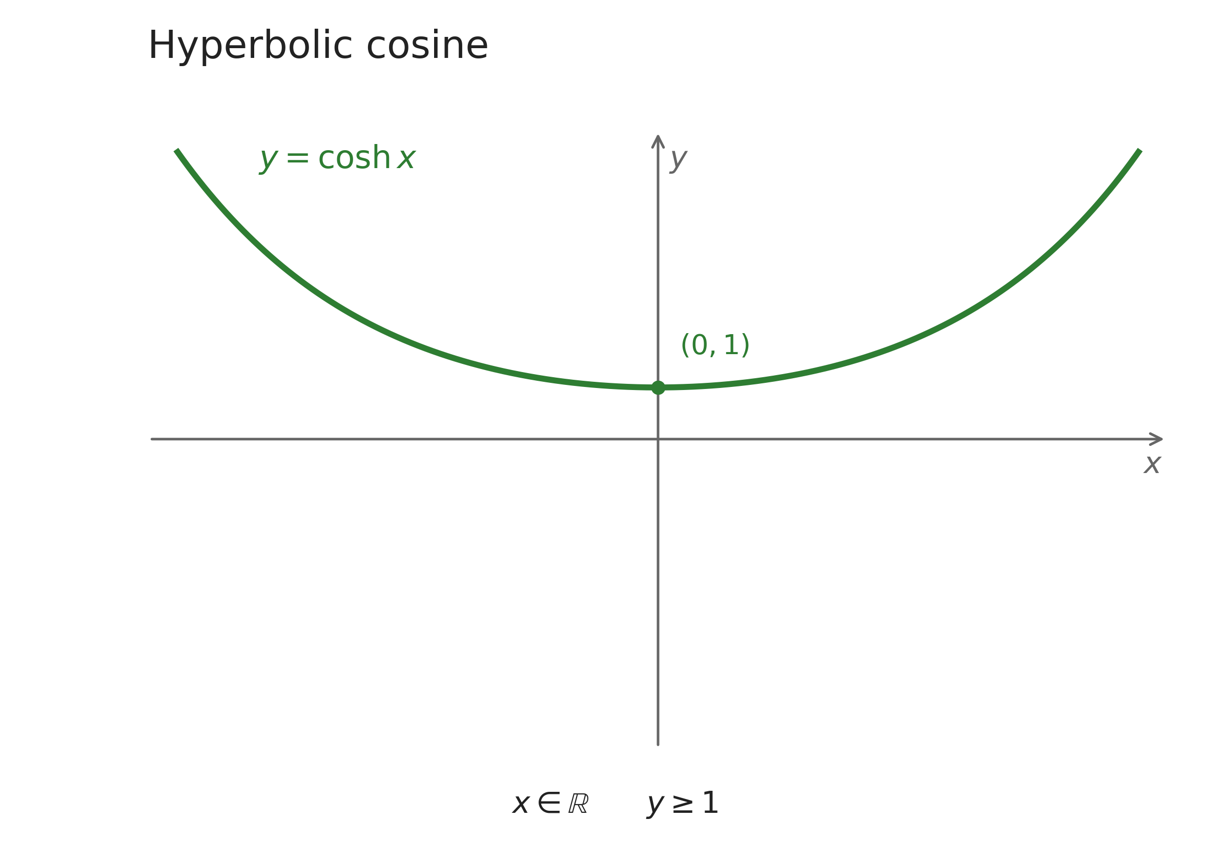
Finally, we can explore the graphs of these hyperbolic functions. Not surprisingly, they are not periodic because they are defined with the hyperbola. When graphed, hyperbolic cosine forms a curve known as a catenary:

Figure 6.7

The catenary curve has an interesting connection with the physical world. Get a piece of rope or wire and let it hang freely while holding it at the same height on both sides. Most people would say that the curve formed by a free-hanging rope makes a parabola.

Figure 6.8

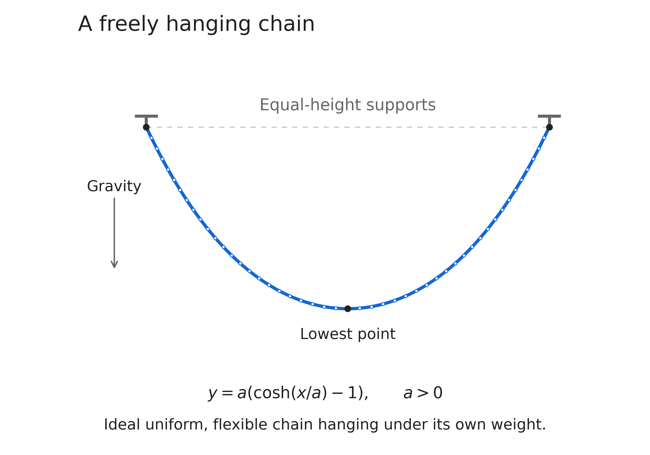
However, it actually forms a scaled version of the catenary curve. While a catenary is similar to a parabola, it will not match up with a parabola at any scale.³

It is the same on both sides of the y-axis because the sign of the area does not matter to the hyperbolic cosine function. The unscaled hyperbolic cosine has a minimum at \((0,1)\), since the x-coordinate is 1 when the hyperbolic sector is just the x-axis and there is no area.

The graph of hyperbolic sine looks like this:

Figure 6.9

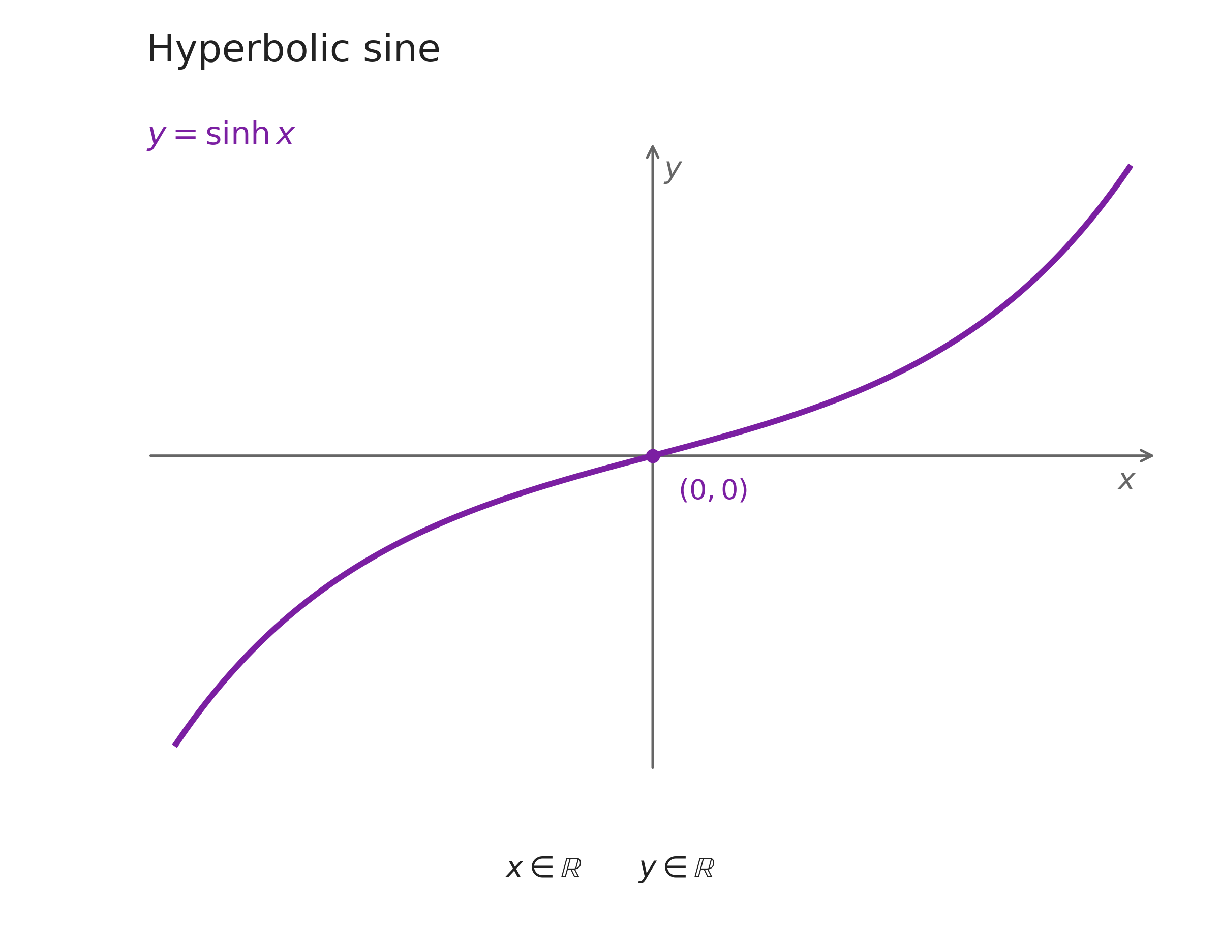
This looks similar to the graph of a cubic equation, but again it is not the graph of any cubic equation.

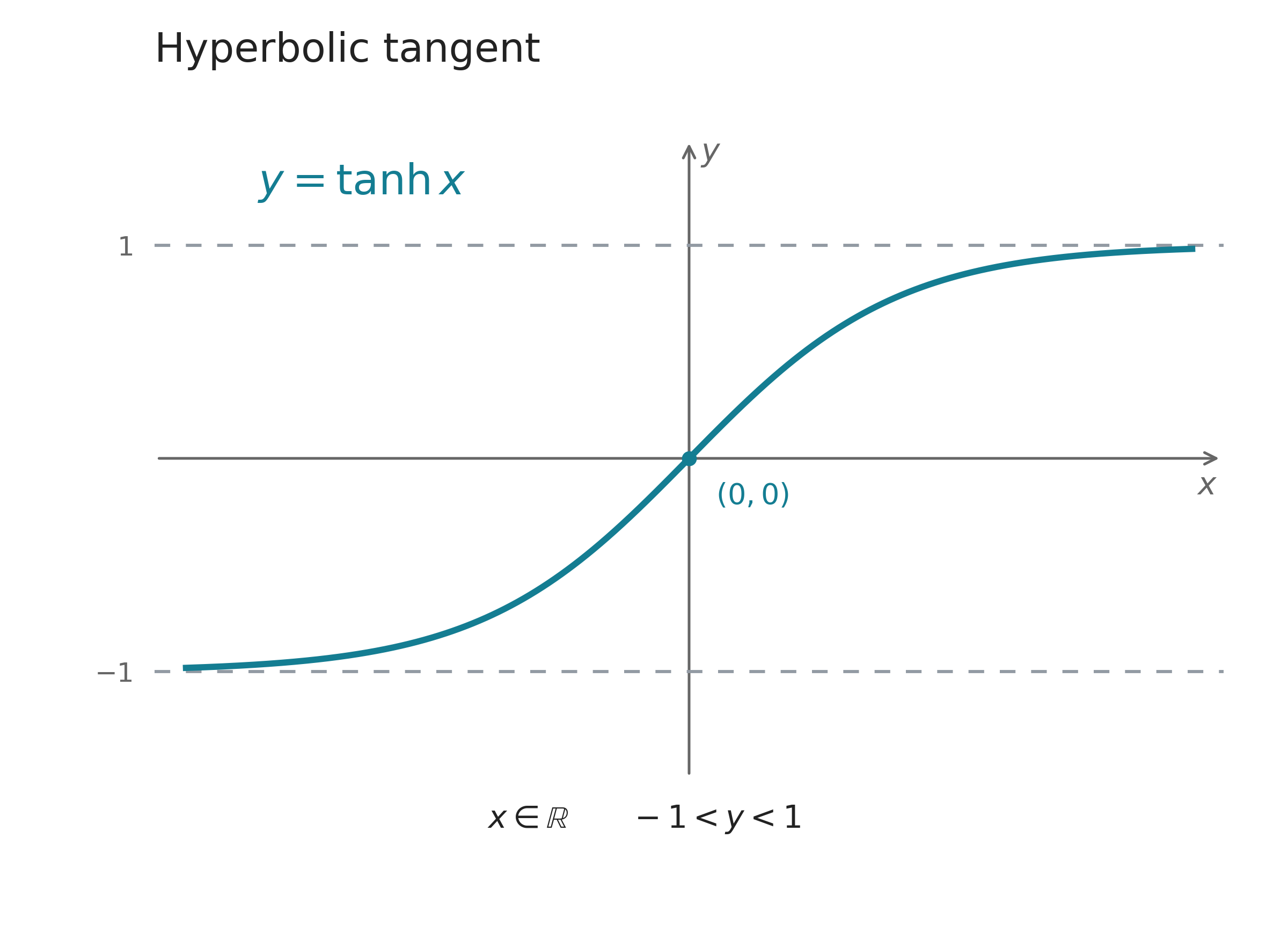
The function \(\tanh(x)\) can’t go above 1, because the hyperbola itself approaches the line \(y = x\). This line has a slope of one, so the slope of a line segment defining a hyperbolic sector cannot be equal to or above 1.

Therefore, \(\tanh(x)\) has an asymptote at \(y = 1\), because the slope will forever get closer and closer to 1. The graph looks like this:

Figure 6.10

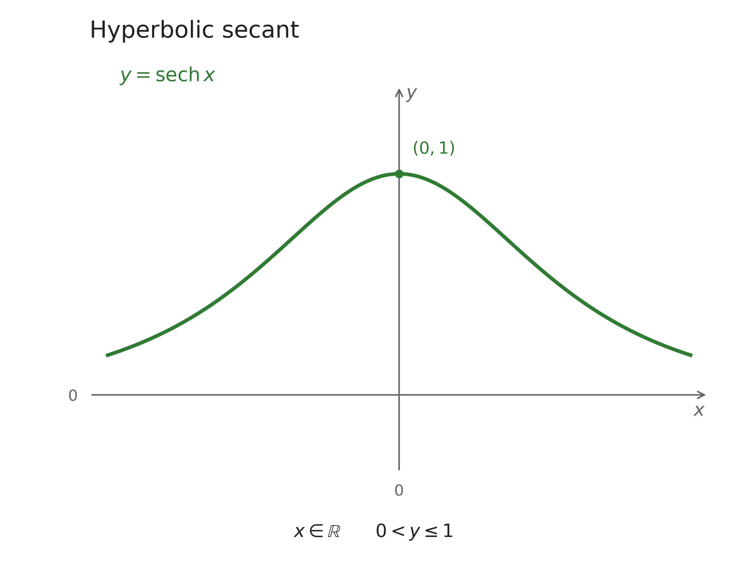
The other functions are simply reciprocals of the first three, but require examining the functions they come from to draw accurate graphs. Starting with hyperbolic secant, we can infer that it approaches zero because its reciprocal (hyperbolic cosine) approaches infinity. Likewise, \(\cosh(x)\) has a minimum at the point \((0,1)\), so this is the maximum of \(sech(x)\). The graph looks like this:

Figure 6.11

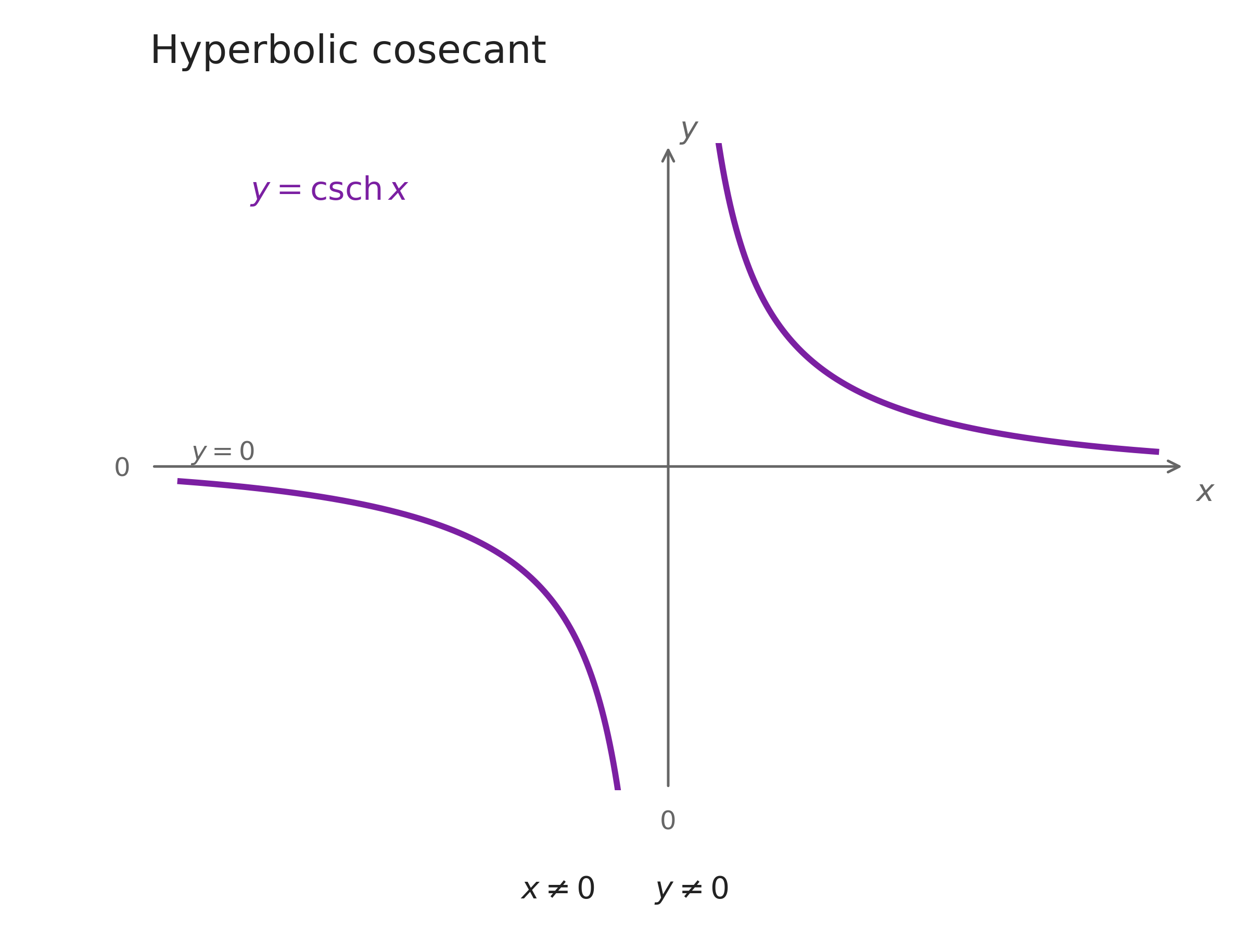
While you might initially expect the graph of hyperbolic cosecant to look something like hyperbolic secant, this is not the case. Because \(\sinh(0) = 0\), the reciprocal will blow up as the input approaches zero. In addition, because hyperbolic sine approaches infinity and negative infinity in their respective directions, the function will approach zero on the x-axis as well. The function looks similar to the reciprocal function \(\frac{1}{x}\), and its graph is:

Figure 6.12

Finally, hyperbolic cotangent is the reciprocal of hyperbolic tangent. The first thing we can notice is that hyperbolic tangent forever approaches 1, so its reciprocal must also approach 1 from the other side. The same can be said on the negative side where both functions approach -1. Second, because \(\tanh(0) = 0\), hyperbolic cotangent will have vertical asymptotes as the x-values approach zero, similar to hyperbolic cosecant.

Figure 6.13

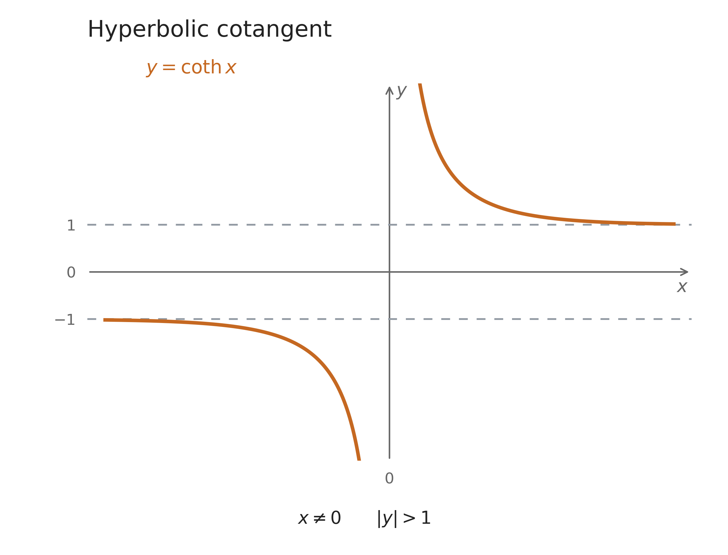
Inverse Hyperbolic Trigonometry

Just as inverse trig functions could be thought of as getting input of a segment on the unit circle and giving back the angle or twice the area, the inverse hyperbolic functions can be extended in the same way.

They are usually denoted by either \(\cosh^{- 1}(x)\) or \(arcosh(x)\), which stands for area hyperbolic cosine (although it really gives twice the area). Given an x-coordinate on the upper half of the right branch of the unit hyperbola, \(arcosh(x) = 2a\), where \(a\) is the nonnegative area of the hyperbolic sector.

Similarly, given a y-coordinate on the right branch, with a taken as the signed area, you can use the area hyperbolic sine function \(arsinh(y) = 2a\). I will use the notation \(arcosh(x)\) for the rest of the book to avoid the confusion with fractions.

We can use the exponential formulas to calculate the inverse functions with logarithms. Start with \(y = sinh\ t\) and write \(E = e^{t}\). Since \(e^{- t} = 1/E\),

\[y = \frac{E - E^{- 1}}{2}\quad \Rightarrow \quad E^{2} - 2yE - 1 = 0.\]

We wanted to find an input to a hyperbolic function, but now we have a quadratic. Multiplying by \(E\) was allowed because an exponential is never zero. We can solve for \(E\) first, then undo \(E = e^{t}\) with a logarithm. Its two roots are

\[E = y \pm \sqrt{y^{2} + 1}.\]

Because \(E = e^{t}\) must be positive, we take the plus sign. The square root is greater than \(|y|\), so this choice is positive even when \(y\) is negative. The minus choice is always negative and cannot be an exponential value. Taking a natural logarithm gives

\[\boxed{arsinhy = ln\left( y + \sqrt{y^{2} + 1} \right)}\]

For \(u = cosht\), we need a restriction: \(\cosh t\) is even, so it cannot tell \(t\) and \(- t\) apart. We choose the principal inverse, which returns \(t \geq 0\) and accepts \(u \geq 1\). With the same substitution,

\[u = \frac{E + E^{- 1}}{2}\quad \Rightarrow \quad E^{2} - 2uE + 1 = 0.\]

This time both quadratic roots are positive. The condition \(t \geq 0\) means \(E \geq 1\), so we choose \(E = u + \sqrt{u^{2} - 1}\). Thus

\[\boxed{arcoshu = ln\left( u + \sqrt{u^{2} - 1} \right),\quad\quad u \geq 1.}\]

For \(u > 1\), the other root is the reciprocal of the first and corresponds to \(- t\). It is not a second value of our chosen inverse. At \(u = 1\), the roots coincide at \(E = 1\), giving \(t = 0\). Both formulas use the nonnegative real square root. Their different input restrictions come from the different ranges of sinh and cosh, not from a choice made by the logarithm.

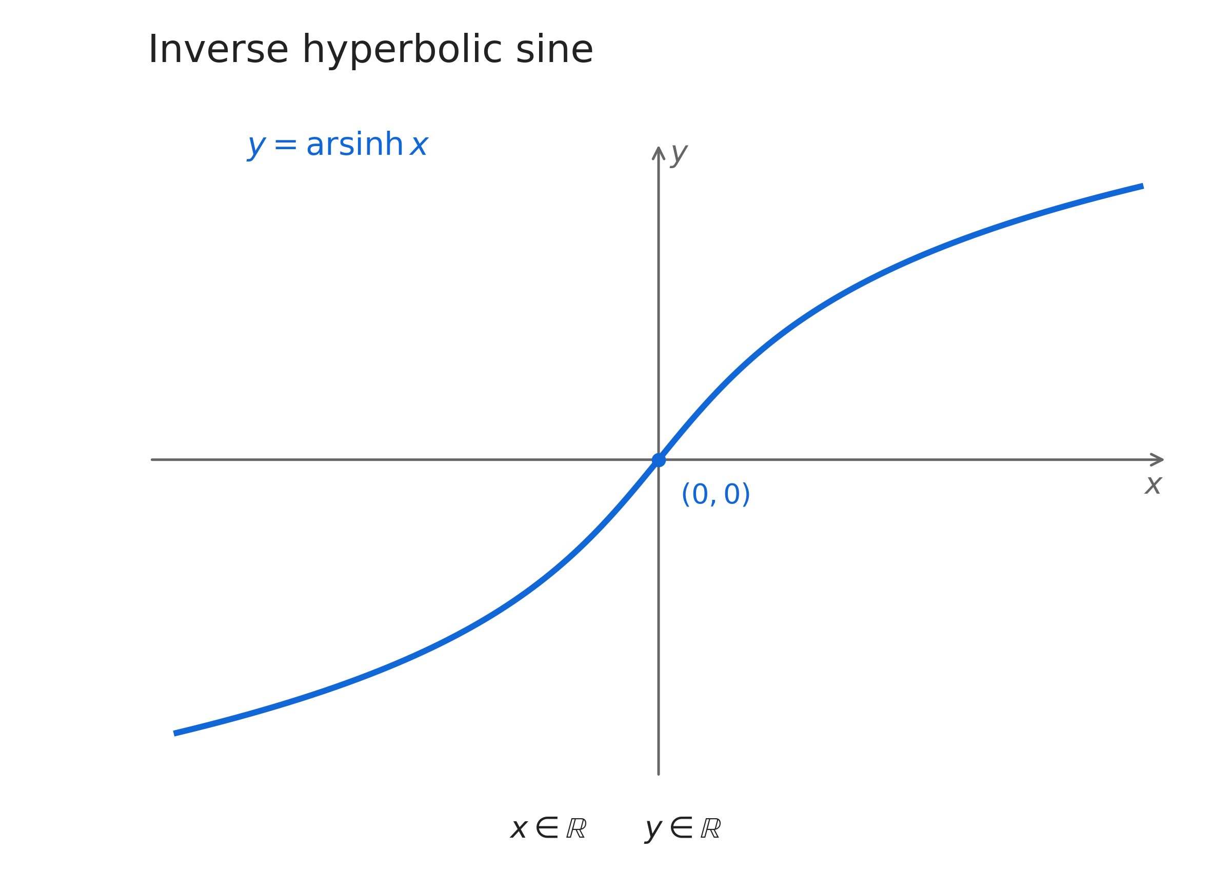
For our inverse hyperbolic functions, \(arsinh(x)\) can accept all values, and simply looks like a sideways version of the original function.

Figure 6.14

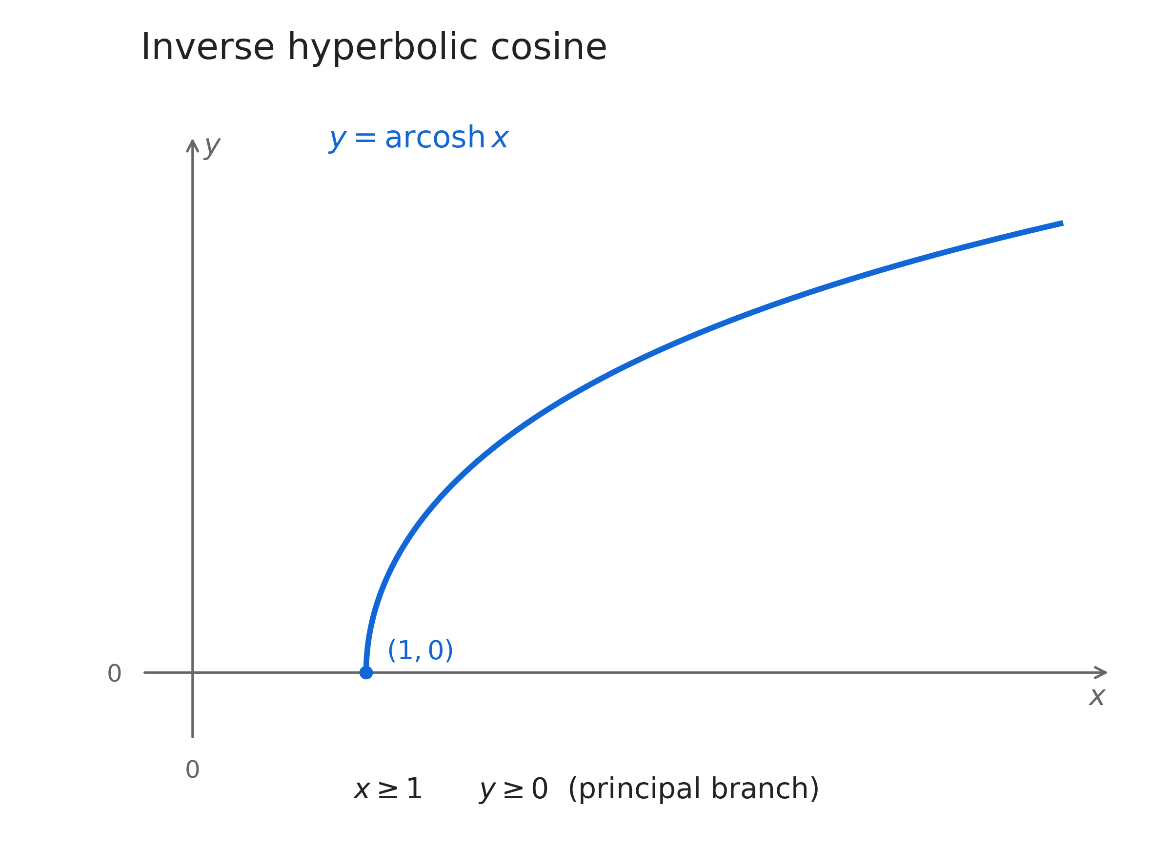
Inverse hyperbolic cosine can only accept values greater than or equal to 1 as input, since \(\cosh(x)\) only outputs values greater than or equal to 1. Also, since \(\cosh( - x) = \cosh(x)\), each input greater than 1 corresponds to two opposite inputs of hyperbolic cosine, while 1 corresponds only to 0. Therefore, we restrict the inverse’s output to nonnegative numbers.

Figure 6.15

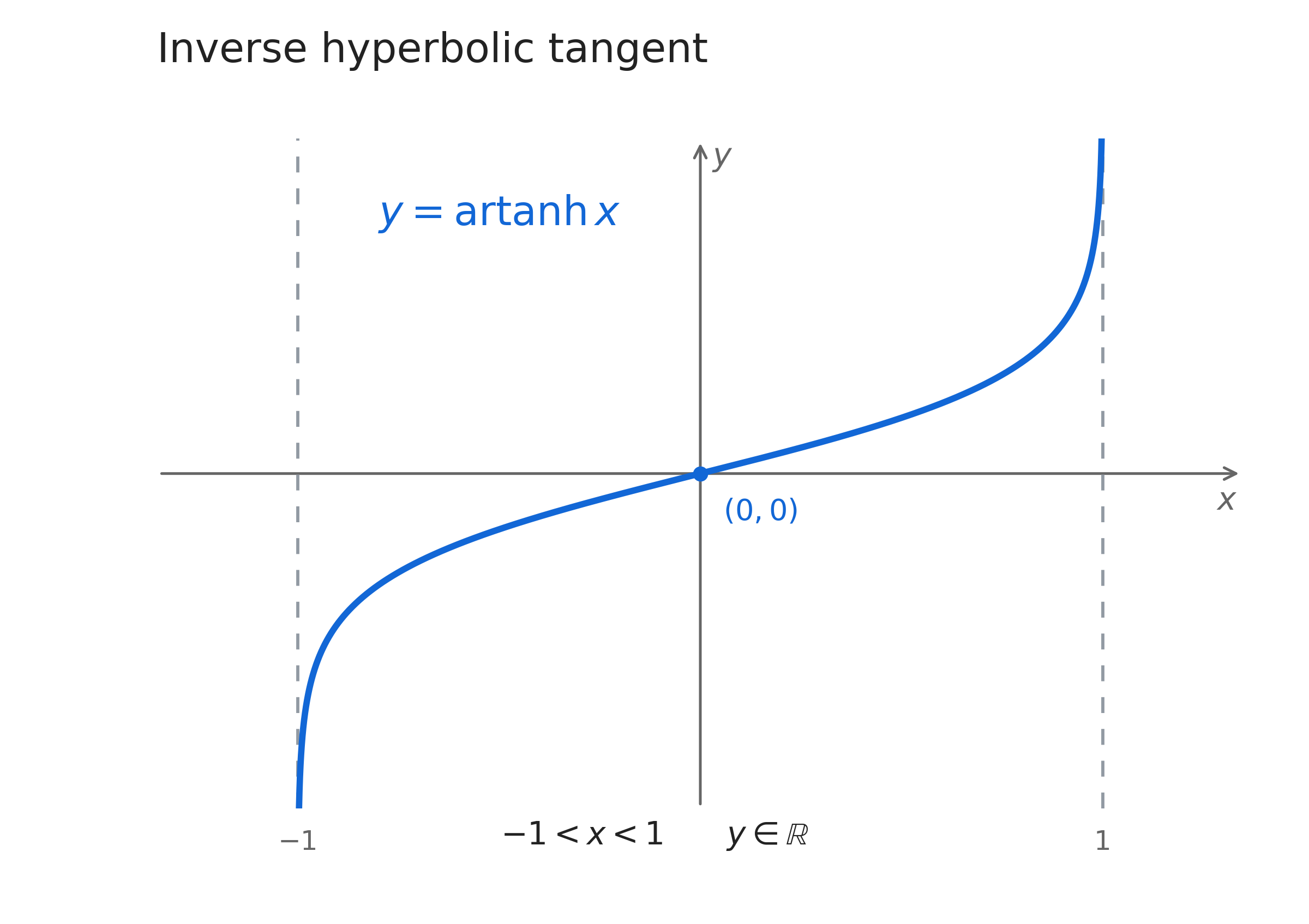
Inverse hyperbolic tangent can only accept values between -1 and 1, and looks like:

Figure 6.16

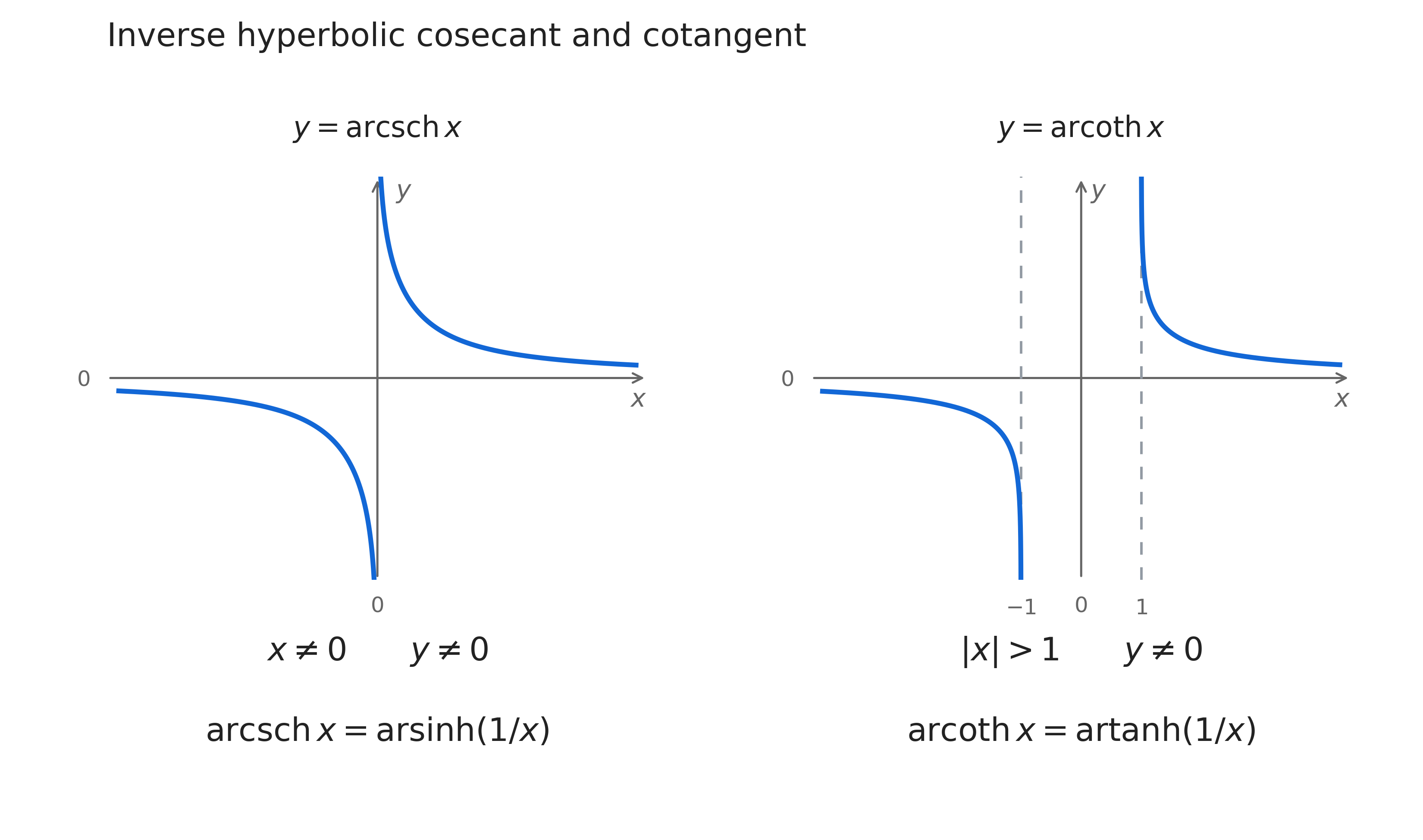
The inverses of hyperbolic cosecant and cotangent look surprisingly similar to the original functions, except that the asymptotes are switched.

Figure 6.17

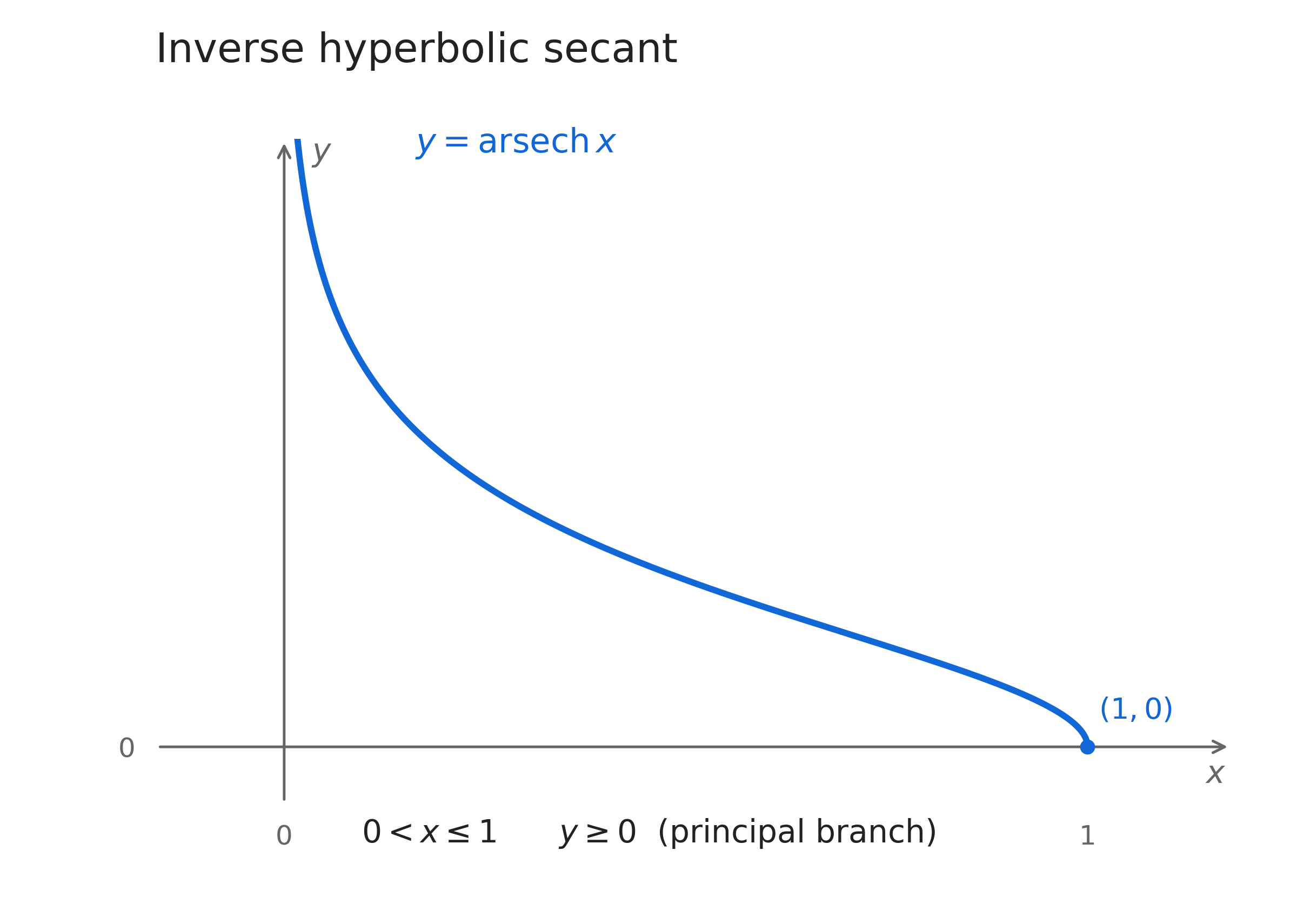
Finally, hyperbolic secant also satisfies \(sech( - x) = sech(x)\), so we must restrict the inverse’s output to nonnegative numbers. In addition, since hyperbolic secant only outputs values greater than 0 and less than or equal to 1, the inverse accepts exactly those inputs. The inverse looks like this:

Figure 6.18

Comparing the Hyperbolic Functions

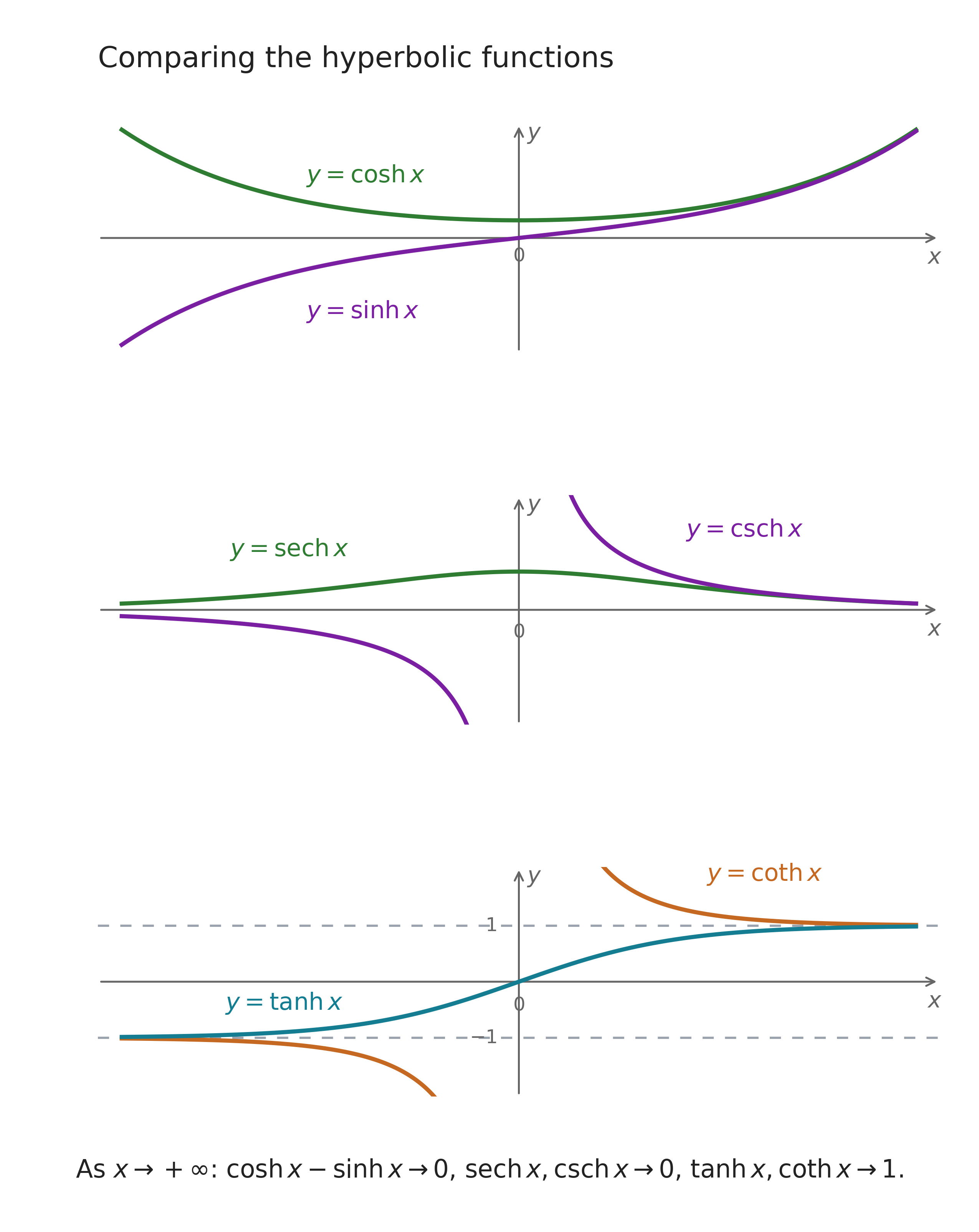
Superimposing the graphs of the six original hyperbolic functions, we can realize some interesting properties of these hyperbolic functions.

First, we can see that hyperbolic sine and cosine approach each other as the x-values grow larger, but this makes sense, since the x and y coordinates on the unit hyperbola approach the line \(y = x\). Likewise, their reciprocals approach each other, because they both have asymptotes at 0. Similarly, hyperbolic tangent and cotangent approach a value of one from opposite sides.

Figure 6.19

Hyperbolic Solution to the Cubic Equation

Similar to how we derived a trigonometric solution to the cubic with three real roots, hyperbolic functions allow us to solve cubics in the case of one real root. The algebra is mostly the same; however, a geometric interpretation of this requires more advanced math than is discussed in this book.

There are actually two different formulas for two cases of one real root. First, for both cases, the quantity under the square root in Cardano’s formula, which we will call \(D,\) must be greater than zero:

\[\left( \frac{q}{2} \right)^{2} + \left( \frac{p}{3} \right)^{3} > 0\]

We use hyperbolic cosines in the case that \(p < 0\), and hyperbolic sines in the case of \(p > 0\).

Solution by Hyperbolic Cosines

Recall that we are solving a depressed cubic,

\[x^{3} + px + q = 0,\quad\quad D = \left( \frac{q}{2} \right)^{2} + \left( \frac{p}{3} \right)^{3} > 0.\]

The classical cubic discriminant is \(- 108D\), so the two quantities have opposite signs.

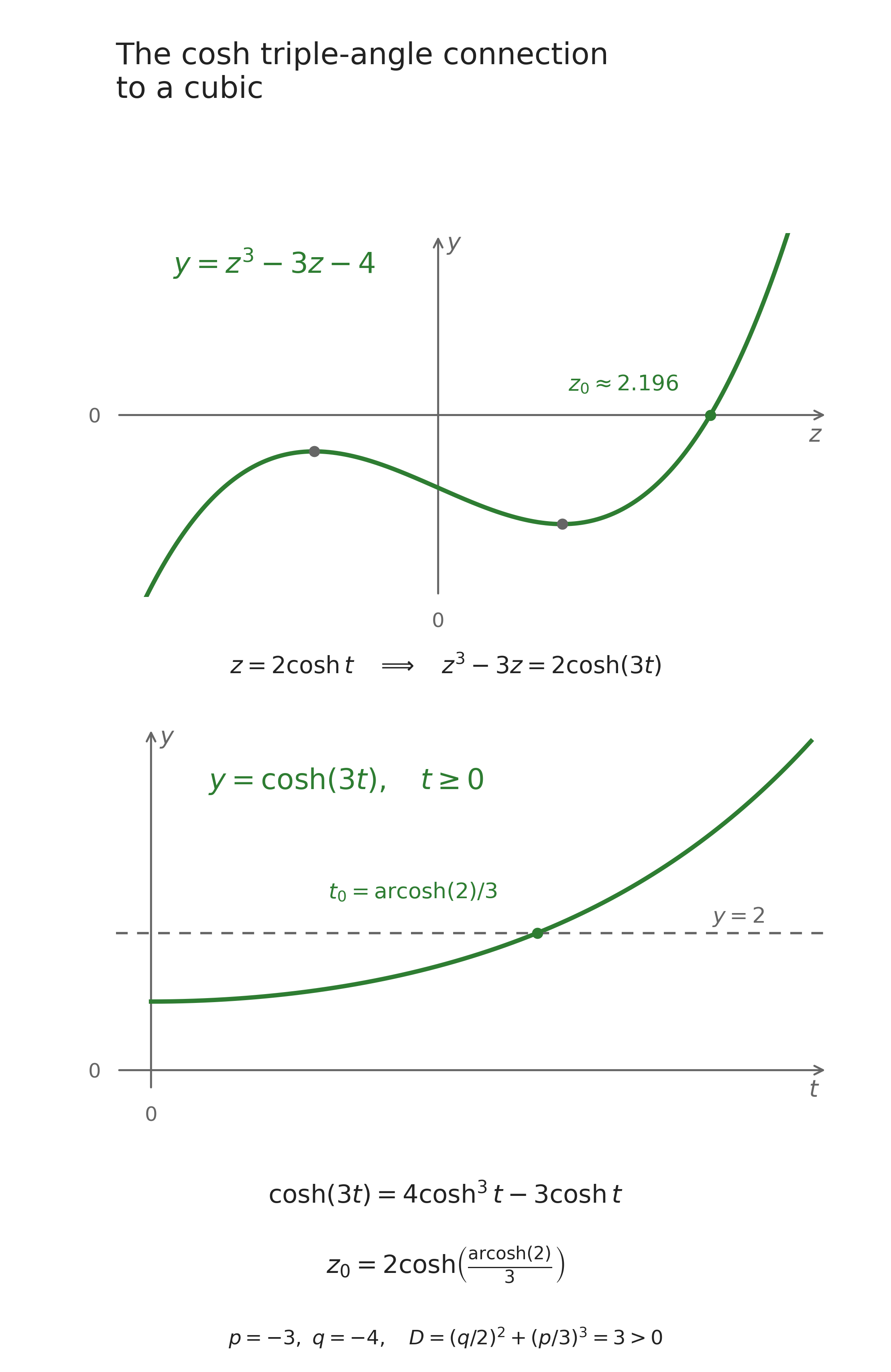
In Chapter 5, we matched the cubic with the cosine triple-angle identity. We can try the same approach with hyperbolic cosine, but first we can derive the identity directly from its exponential formula. Cubing gives

\[4\cosh^{3}t = \frac{e^{3t} + 3e^{t} + 3e^{- t} + e^{- 3t}}{2}\]

Subtracting \(3\cosh t\) cancels the middle two terms:

\[\boxed{4\cosh^{3}t - 3\cosh t = \frac{e^{3t} + e^{- 3t}}{2} = cosh(3t)}\]

This has the cubic term and negative linear term we need.

Suppose \(p < 0\), and set \(a = \sqrt{- p/3}\), so \(p = - 3a^{2}\) and \(a > 0\). The factor \(2a\) will make the ratio of the cubic and linear coefficients match the ratio in our identity. We are choosing a scale for the substitution, just as we did for ordinary cosine.

There is one sign to keep track of. Hyperbolic cosine is always positive, but the root we want can be negative.

Let \(s = - sgn(q)\), meaning \(s = 1\) when \(q < 0\) and \(s = - 1\) when \(q > 0\).

We will see below that \(q = 0\) cannot occur in this case.

Now substitute

\[x = 2as\ \cosh\ t,\quad\quad t \geq 0\]

Because \(s^{3} = s\), the cubic and linear terms become

\[x^{3} + px = 8a^{3}s\ \cosh^{3}t - 6a^{3}s\ \cosh\ t\]

Factoring out \(2a^{3}s\) gives

\[x^{3} + px = 2a^{3}s\left( 4\cosh^{3}t - 3\cosh\ t \right) = 2a^{3}s\ \cosh(3t).\]

To make this equal \(- q\), we therefore need

\[\cosh(3t) = \frac{|q|}{2a^{3}}.\]

This is also why we chose \(s\) opposite in sign to \(q\): the remaining cosh factor is positive. We must still check that the right side is a possible cosh value. Since

\[D = \frac{q^{2}}{4} - a^{6} > 0\]

we have \(|q| > 2a^{3}\). In particular, \(q \neq 0\), and the inverse-cosh input is greater than one. An ordinary cosine could not equal this number: its values stop at one. Hyperbolic cosine starts at one and grows without bound on nonnegative inputs, so it gives us exactly the range we need here. Restricting \(t\) to be nonnegative avoids counting the same cosh value twice. Taking the principal inverse gives

\[t = \frac{1}{3}arcosh\left( \frac{|q|}{2a^{3}} \right).\]

Substituting back,

\[\boxed{x = - 2a\, sgn(q)\,\cosh\left( \frac{1}{3}arcosh\left( \frac{|q|}{2a^{3}} \right) \right),\quad\quad a = \sqrt{- p/3}}\]

This gives the unique real root when \(p < 0\) and \(D > 0\). Its sign comes entirely from the factor in front of cosh. A negative \(q\) therefore gives a positive answer, and a positive \(q\) gives a negative answer.

The repeated-root boundary \(D = 0\) and the three-distinct-real-root case \(D < 0\) belong to the earlier cubic treatment. If we began with \(z^{3} + bz^{2} + cz + d = 0\), we finally undo the earlier shift using \(z = x - b/3\).

Figure 6.20

Solution by Hyperbolic Sines

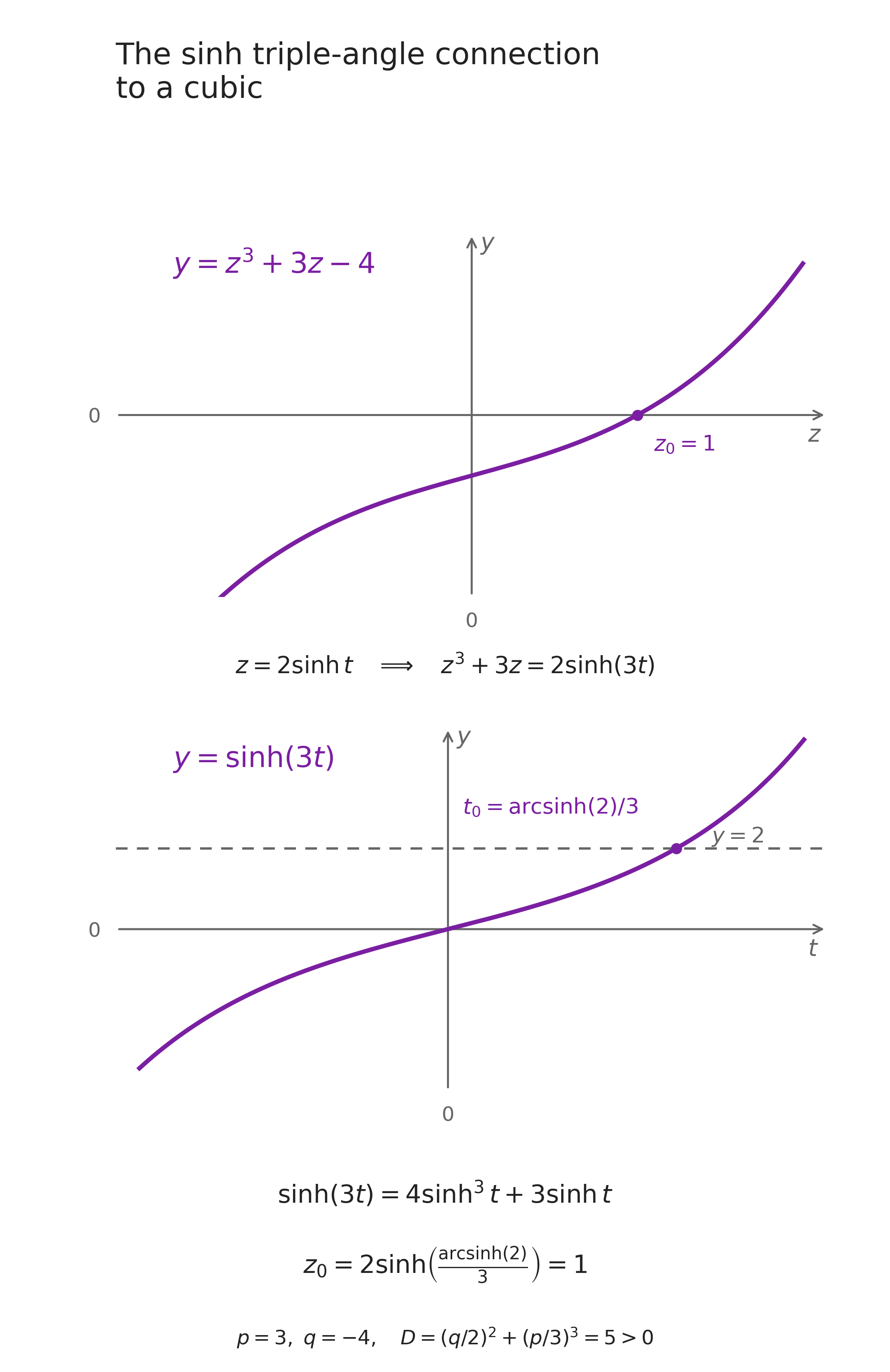
When \(p > 0\), the linear term has the wrong sign for the cosh identity. Hyperbolic sine gives us the other sign. Cubing its exponential expression produces

\[4\sinh^{3}t = \frac{e^{3t} - 3e^{t} + 3e^{- t} - e^{- 3t}}{2}\]

Now we add \(3\sinh\ t\) to cancel the middle terms:

\[\boxed{4\sinh^{3}t + 3\sinh\ t = \frac{e^{3t} - e^{- 3t}}{2} = sinh(3t).}\]

The same coefficient matching suggests \(a = \sqrt{p/3}\), so \(p = 3a^{2}\), and the substitution \(x = 2a\sinh t\). We keep the scale positive and allow \(t\) itself to be any real number. Unlike cosh, sinh can provide the negative values without an extra factor in front. This gives

\[x^{3} + px = 8a^{3}\sinh^{3}t + 6a^{3}\sinh\ t\]

Factoring out \(2a^{3}\) gives

\[x^{3} + px = 2a^{3}\left( 4\sinh^{3}t + 3\sinh\ t \right) = 2a^{3}\sinh(3t).\]

Setting this equal to \(- q\) leaves

\[\sinh(3t) = - \frac{q}{2a^{3}},\quad\quad t = \frac{1}{3}arsinh\left( - \frac{q}{2a^{3}} \right).\]

Here we do not need a separate sign factor. Hyperbolic sine takes every real value exactly once, so its inverse accepts any real input, positive, negative or zero. There is no requirement that the magnitude of the inverse input exceed one. That restriction belonged to cosh; carrying it into this case would wrongly exclude valid cubics. Also, \(a > 0\), so the denominator is never zero. Substituting back gives

\[\boxed{x = 2a\,\sinh\left( \frac{1}{3}arsinh\left( - \frac{q}{2a^{3}} \right) \right),\quad\quad a = \sqrt{p/3}}\]

Because \(p > 0\), the quantity \(D = (q/2)^{2} + (p/3)^{3}\) is positive for every real \(q\). This is therefore the unique real root throughout this case. If \(q > 0\), the inverse input and the answer are negative; if \(q < 0\), both are positive. When \(q = 0\), the formula gives

\[x = 2a\sinh(0) = 0\]

As before, if we removed a quadratic term at the start, we finish by shifting back to the original variable.

Figure 6.21

The Zero-Coefficient Case

There is one case left: \(p = 0\). We cannot use either normalized formula here, because \(a\) would be zero and appear in the denominator. But the equation itself is much simpler:

\[x^{3} + q = 0,\quad\quad x = \sqrt[3]{- q}.\]

We take the real cube root, keeping its sign. If \(q \neq 0\), this is the unique real root and \(D = q^{2}/4 > 0\). If \(q = 0\) as well, the equation is \(x^{3} = 0\): zero is a triple root, and \(D = 0\), outside the strictly positive-\(D\) cases above.

A Worked Example

Let’s use the formula to solve

\[x^{3} - 3x - 18 = 0.\]

Here \(p = - 3\) and \(q = - 18\), so

\[D = ( - 9)^{2} + ( - 1)^{3} = 80 > 0,\quad\quad a = \sqrt{- p/3} = 1\]

Since \(p < 0\), we use hyperbolic cosine. Since \(q < 0\), the root has a positive sign. Substituting into the formula gives

\[x = 2\cosh\left( \frac{1}{3}arcosh(9) \right)\]

We can evaluate this exactly using the same triple-angle identity. The expression asks us to find an input whose triple gives a cosh value of nine. Rather than introduce rounding, we can check a possible value of cosh at the smaller input. Take the nonnegative \(t\) for which \(\cosh t = 3/2\). Then

\[\cosh(3t) = 4\left( \frac{3}{2} \right)^{3} - 3\left( \frac{3}{2} \right) = 9\]

Because \(3t \geq 0\), it follows that \(arcosh9 = 3t\).

Our answer is therefore

\[x = 2\cosh t = 3\]

Now we can check the answer without using any hyperbolic functions. Direct substitution gives \(27 - 9 - 18 = 0\). Factoring gives

\[x^{3} - 3x - 18 = (x - 3)\left( x^{2} + 3x + 6 \right)\]

The remaining quadratic has discriminant \(3^{2} - 4(1)(6) = - 15\).

It has no real roots, so \(3\) really is the only real root of the original cubic. The formula has found the root, and ordinary algebra has checked both the value and the number of real solutions.

Toward Complex Numbers

In Chapter 5, the cosine triple-angle identity gave us a route to three distinct real roots. Hyperbolic cosine and sine have now handled the cases where \(D > 0\) and there is only one real root, with \(p = 0\) handled directly. The repeated-root boundary remains a separate case.

For \(x^{3} - 3x - 18 = 0\), we found the real root and were left with a quadratic whose discriminant was negative. To find its other roots, real numbers are no longer enough. The next step is to enlarge the number system.

← Previous chapter Book contents Next chapter →

Footnotes

1. Gyula Pápay, “Mercator’s Geometric Method in the Construction of His Projection from 1569,” KN – Journal of Cartography and Geographic Information 72 (2022): 261–67, https://doi.org/10.1007/s42489-022-00115-5; J. J. O’Connor and E. F. Robertson, “Vincenzo Riccati,” MacTutor History of Mathematics Archive, University of St Andrews, accessed October 15, 2026, https://mathshistory.st-andrews.ac.uk/Biographies/Riccati_Vincenzo/; Florian Cajori, A History of Mathematical Notations, vol. 2, Notations Mainly in Higher Mathematics (Chicago: Open Court Publishing Company, 1929), 172.

2. G. Osborn, “109. [D. 6. d.] Mnemonic for Hyperbolic Formulae,” The Mathematical Gazette 2, no. 34 (July 1902): 189, https://doi.org/10.2307/3602492.

3. F. Behroozi, “A Fresh Look at the Catenary,” European Journal of Physics 35, no. 5 (2014): 055007, https://doi.org/10.1088/0143-0807/35/5/055007.