Chapter 4: Trigonometry
The search for polynomial formulas has shown us how much we can do with arithmetic and radicals. We can also ask what other functions might help us understand equations. We will begin with functions defined by a circle, then see how they lead us back to the cubic.
Circular Trigonometry
Basic Definitions
While most mathematics classes and books first present trigonometry in terms of right triangles (which makes sense because trigonometry literally translates to “triangle measure”)1, I will instead present the trigonometric functions in terms of the unit circle.
The unit circle is the circle on a coordinate plane with a center at (0,0) and a radius of 1.
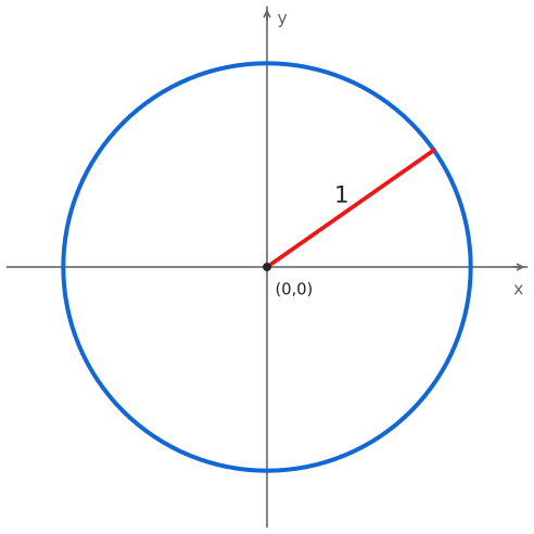
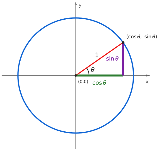
The cosine and sine functions take an angle, call it \(\theta\), and draw a radius from the origin to the unit circle at that angle, measured counterclockwise from the positive x-axis. The cosine of an angle is the x-coordinate of the point, while the sine is the y-coordinate of the point.
Those of you who learned “SOHCATOA” trigonometry may ask, “how does this connect to the right triangles?” Take an angle \(\theta\) between \(0^{\circ}\) and \(90^{\circ}\), and drop a perpendicular from its point on the unit circle to the x-axis. The radius is the hypotenuse, with length one. The adjacent side has length \(\cos\theta\), and the opposite side has length \(\sin\theta\).
If we enlarge this triangle by any positive factor \(r\), all three sides scale together. Dividing either leg by the hypotenuse cancels that factor, giving
\[\boxed{\cos\theta = \frac{\text{adjacent side}}{\text{hypotenuse}},\quad\quad\sin\theta = \frac{\text{opposite side}}{\text{hypotenuse}}}\]
So the two definitions agree for acute angles. The circle also lets us keep going beyond those angles, using signed coordinates instead of just positive side lengths.
Because adding 360° to an angle doesn’t change its relative position on the circle, the sine and cosine functions are the same for any angle added to 360°. This means that the functions have the exact same behavior when you add or subtract multiples of 360°.
Another observation is that, when we take the angle formed with the y-axis (assuming the angle is between 0 and 90°), which is known as the complementary angle, the sine and cosine segments flip. This angle is \(90^{{^\circ}} - \theta\), so therefore we can derive that
\[\sin\left( 90^{{^\circ}} - \theta \right) = cos(\theta) \qquad\text{and}\qquad \cos\left( 90^{{^\circ}} - \theta \right) = \sin(\theta)\]
In fact, this is where the cosine function got its name, as it is a shortening of the phrase “complement sine”, meaning the sine of the complementary angle.2
We can also extend these functions to negative-valued angles, by defining them as going the opposite way around the circle, clockwise instead of counterclockwise.
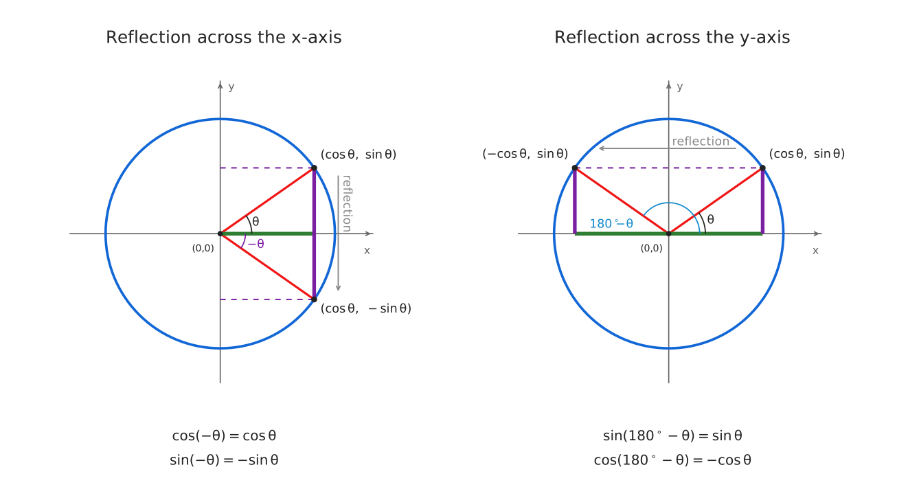
Any negative-valued angle \(- \theta\) has a positive coterminal angle \(- \theta + 360^{\circ}k\), where \(k\) is an integer chosen large enough. These are different angle measures that end at the same point on the circle. The negative of any angle can also be visualized as reflecting the angle over the x-axis. This doesn’t change the x-coordinate, so \(\cos( - \theta) = \cos(\theta)\). The y-coordinate is simply the negative of the original, so \(\sin( - \theta) = - \sin(\theta).\ \)
Reflecting an angle over the y-axis is equivalent to taking \(180^{{^\circ}} - \theta\). Just as reflecting over the x-axis did not change the cosine of an angle, reflecting over the y-axis does not change the sine of an angle. Therefore \(\sin\left( 180^{{^\circ}} - \theta \right) = \sin(\theta)\).
The x-coordinate is on the opposite side of the y-axis from where it started before, so \(\cos\left( 180^{{^\circ}} - \theta \right) = - \cos(\theta)\).
There is another related function to our two original functions, called the tangent function. This function tells us the slope of a line relative to its angle. Because sine tells us our y-coordinate on the unit circle and cosine tells us our x-coordinate,
\[\boxed{\tan(\theta) = \frac{sin(\theta)}{cos(\theta)}}\]
It is worth mentioning that when the cosine of an angle is 0, the tangent function is undefined. This occurs at 90° and 270° (and multiples of 360 added to those measures).
There are three other trigonometric functions that are used less often but are still worth knowing. They are related by reciprocals wherever those reciprocals are defined. The cosecant function is simply
\[\csc(\theta) = \frac{1}{sin(\theta)}\]
Likewise, the secant and cotangent functions are
\[\sec(\theta) = \frac{1}{cos(\theta)} \qquad\text{and}\qquad \cot(\theta) = \frac{\cos(\theta)}{\sin(\theta)}\]
Cosecant and cotangent are undefined when sine is zero, and secant is undefined when cosine is zero. Cotangent is also the reciprocal of tangent when tangent is defined and nonzero; the cosine-over-sine definition still works when cosine is zero.
There is one more amazing fact about the sine and cosine functions that I must mention. The unit circle is defined by the equation \(x^{2} + y^{2} = 1\).
But we can express \(x\) and \(y\) in terms of sine and cosine of an angle, so
\[\boxed{\cos^{2}(\theta) + \sin^{2}(\theta) = 1}\]
This formula will work for any angle \(\theta\), and is one of the simplest and best connections between the cosine and sine functions.
Radian Measure
Up to this point in this chapter, we have been measuring angles in degrees, where 360 degrees is a complete revolution around a circle. However, in many areas of higher mathematics, it is more natural and convenient to describe angles in terms of a measure known as radians. On a unit circle, a radian is defined such that one radian corresponds to a length of one on the circumference of the circle.
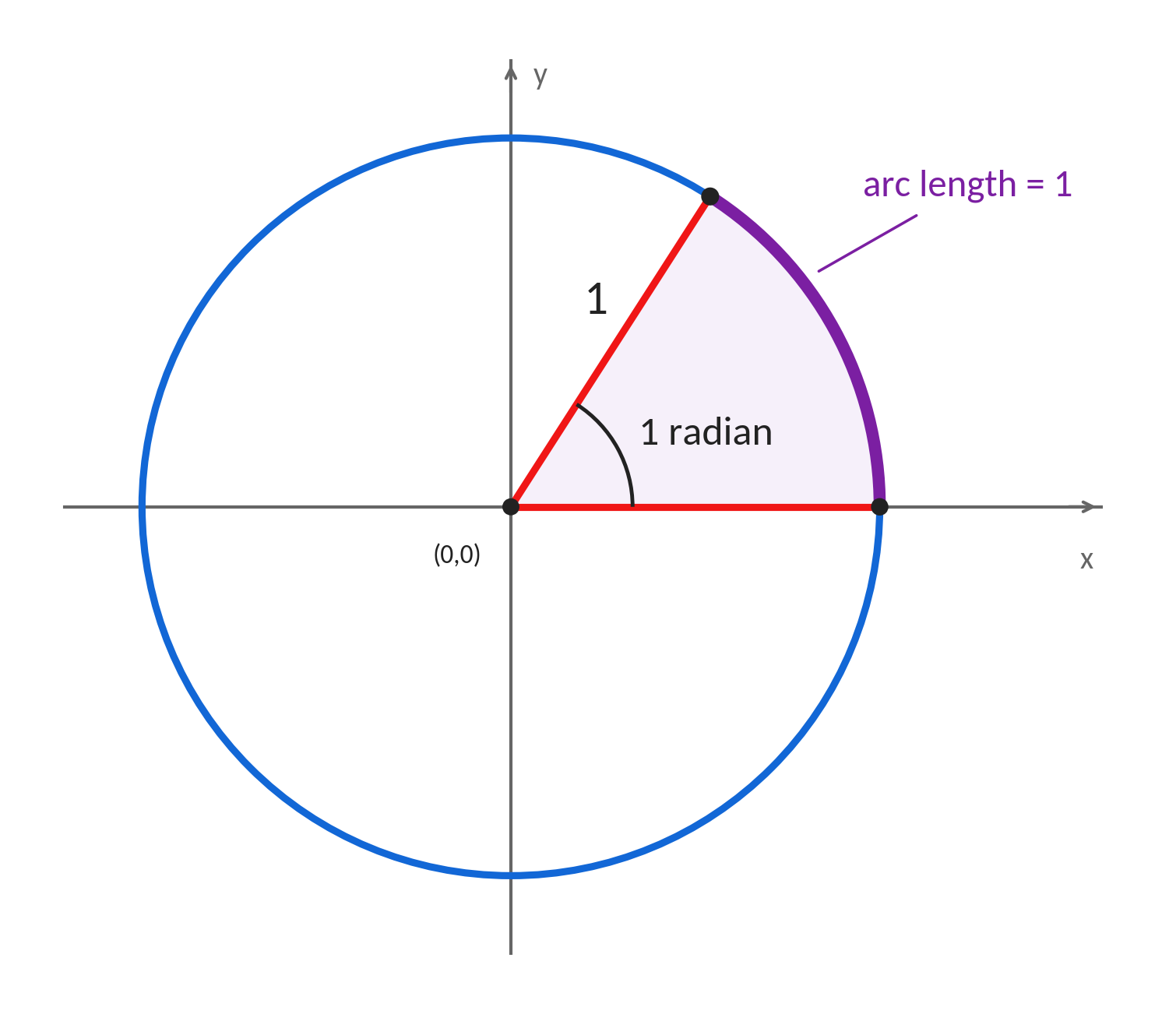
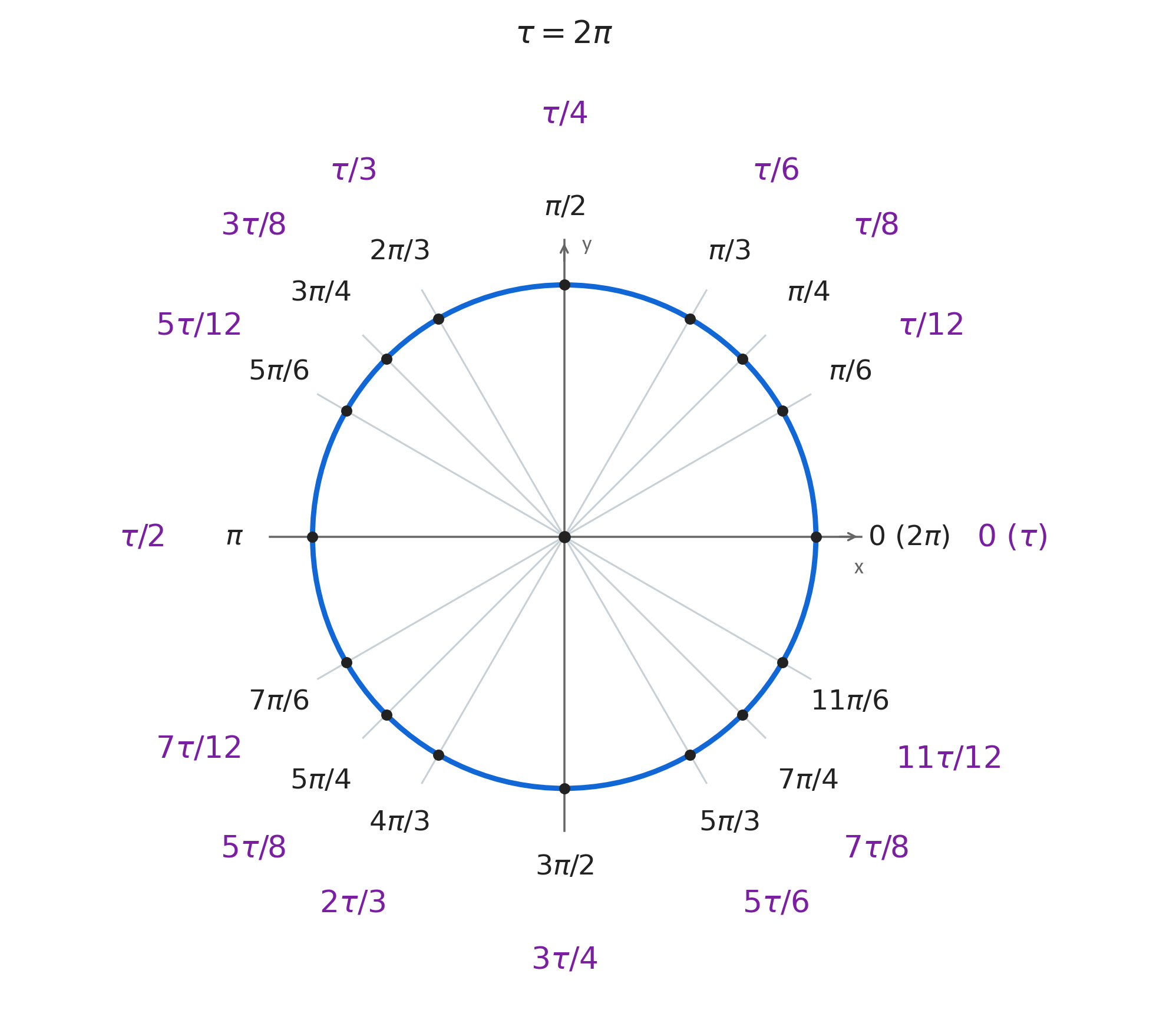
Because the unit circle has a circumference of 2π units, 2π radians is one complete revolution. Thus, 2π radians = 360°. When working in radians, you often come across factors of \(\pi\) multiplied by 2. There is a related constant, called \(\tau\), which is simply 2π. So a full circle is \(\tau\) radians. This makes the math related to radian measure much simpler, because half of a circle is \(\frac{\tau}{2}\) radians, and one third of a circle is \(\frac{\tau}{3}\) radians. This gets rid of all the clunky factors of 2 if we had used \(\pi\). Here is a unit circle with all of the angles expressed in terms of radians. I included the measures in both \(\pi\) and \(\tau\), but I think you will find the \(\tau\) version easier to understand.
Three Angles, Two Triangles
A few angles appear again and again in trigonometry, but their values do not need to be memorized.
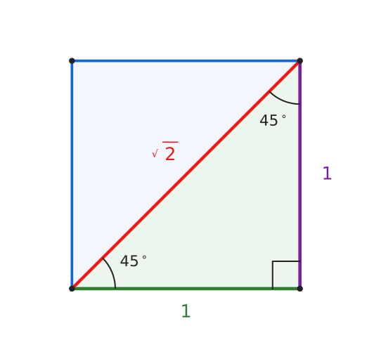
Start with a square whose sides have length \(1\). A diagonal cuts it into two right triangles with angles of \(45^{\circ}\), \(45^{\circ}\), and \(90^{\circ}\). The Pythagorean theorem gives the diagonal length \(\sqrt{2}\), so \(\sin\ 45^{\circ} = cos{\ 45}^{\circ} = 1/\sqrt{2} = \sqrt{2}/2\). In radians, this angle is \(\tau/8\), one eighth of a full turn.
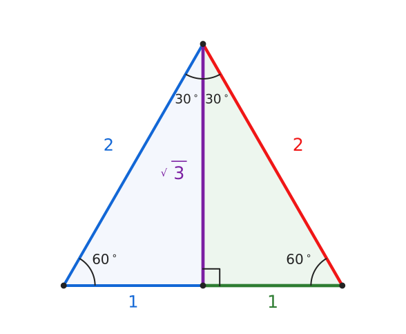
For \(30^{\circ}\) and \(60^{\circ}\), start instead with an equilateral triangle whose sides have length \(2\). Draw an altitude from one vertex to the opposite side. It divides the triangle into two right triangles, each with hypotenuse \(2\), short leg \(1\), and long leg \(\sqrt{3}\). We can read the values straight from that triangle: \(\sin 30^{\circ} = 1/2\), \(\cos 30^{\circ} = \sqrt{3}/2\), \(\sin 60^{\circ} = \sqrt{3}/2\), and \(\cos 60^{\circ} = 1/2\). The corresponding angles are \(\tau/12\) and \(\tau/6\).
Now suppose we want to find sine and cosine at \(210^{\circ}\). That angle is \(30^{\circ}\) past a half-turn, so its reference angle is \(30^{\circ}\). But the point is in the third quadrant, where both coordinates on the unit circle are negative. Therefore \(\sin 210^{\circ} = - 1/2\) and \(\cos 210^{\circ} = - \sqrt{3}/2\). We have used two simple triangles and the signs of the coordinates to calculate values well beyond those first three angles.
Diagram of All 6 Trigonometric Functions
There is an amazing visualization of all six trigonometric functions on the unit circle, but it requires a little bit of work to get there first. For this length construction, take \(0 < \theta < \tau/4\). If we draw the tangent line perpendicular to the radius at its point on the circle, like this:
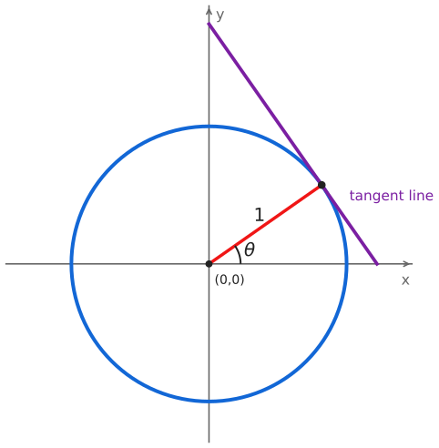
Then we can get two similar triangles, Δ1 and Δ2. I will say the hypotenuse of Δ2 has a length \(D\). I will call the complement of \(\theta\) \(\varphi\)
. Then we can transfer the angles like this:
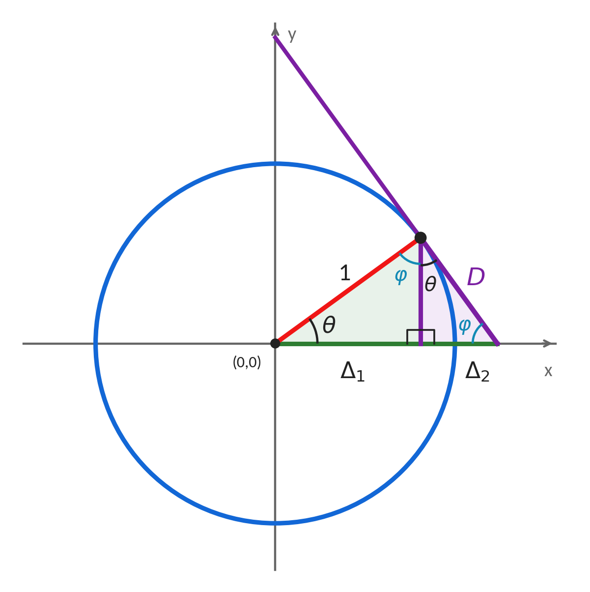
Because of similar triangles, the ratios of the lengths opposite the right angles (\(D\) and 1) must be equal to the ratios of the corresponding legs adjacent to θ (sin θ in Δ2 and cos θ in Δ1).
\[\frac{D}{1} = \frac{sin(\theta)}{cos(\theta)}\]
but we already know that
\[\tan(\theta) = \frac{sin(\theta)}{cos(\theta)}\]
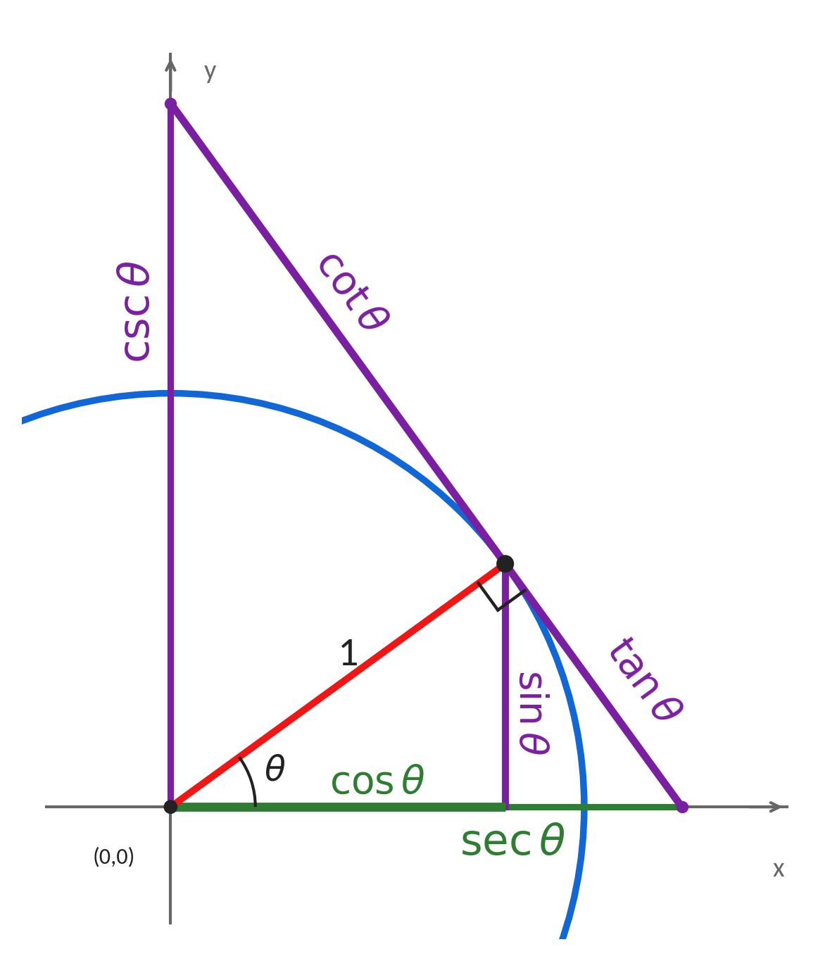
so our distance of \(D\) must be \(\tan(\theta)\). Great!
Following the same logic by similar triangles, we can equate ratios like this
\[\frac{C}{sin(\theta)} = \frac{sin(\theta)}{cos(\theta)}\]
where \(C\) is the unknown side of Δ2. I won’t simplify into tangent for now, because we will need to keep everything in terms of cosine. Multiplying through by \(sin(\theta)\), we obtain
\[C = \frac{\sin^{2}(\theta)}{\cos(\theta)}\]
From our identity \(\sin^{2}(\theta) + \cos^{2}(\theta) = 1\), we can rewrite the numerator because \(\sin^{2}(\theta) = 1 - \cos^{2}(\theta)\). After substituting:
\[C = \frac{1 - \cos^{2}(\theta)}{cos(\theta)}\]
Splitting up the fraction gives
\[C = \frac{1}{cos(\theta)} - \cos(\theta)\]
Then we can rewrite the fraction using reciprocal identities
\[C = \sec(\theta) - cos(\theta)\]
The total length from the origin to the farthest point on the x-axis would be \(C + \cos(\theta)\), so our total length must be \(sec(\theta)\). Awesome!
We can use the same techniques to find that on the other side, the lengths are simply the “co” versions of what we derived before. Combining all of this into a single picture, we have this amazing visual connection between all six trig functions.
Graphs of Trigonometric Functions
For our next exploration of these wonderful trigonometric functions, we will look at what these functions’ graphs look like. The angles will be in radians.
The sine and cosine functions can be thought of as varying up and down as a point moves around the unit circle. There are a lot of great animations of this, but unfortunately I cannot show them in a book. These functions form waves that repeat every \(\tau\) units, and look like this.
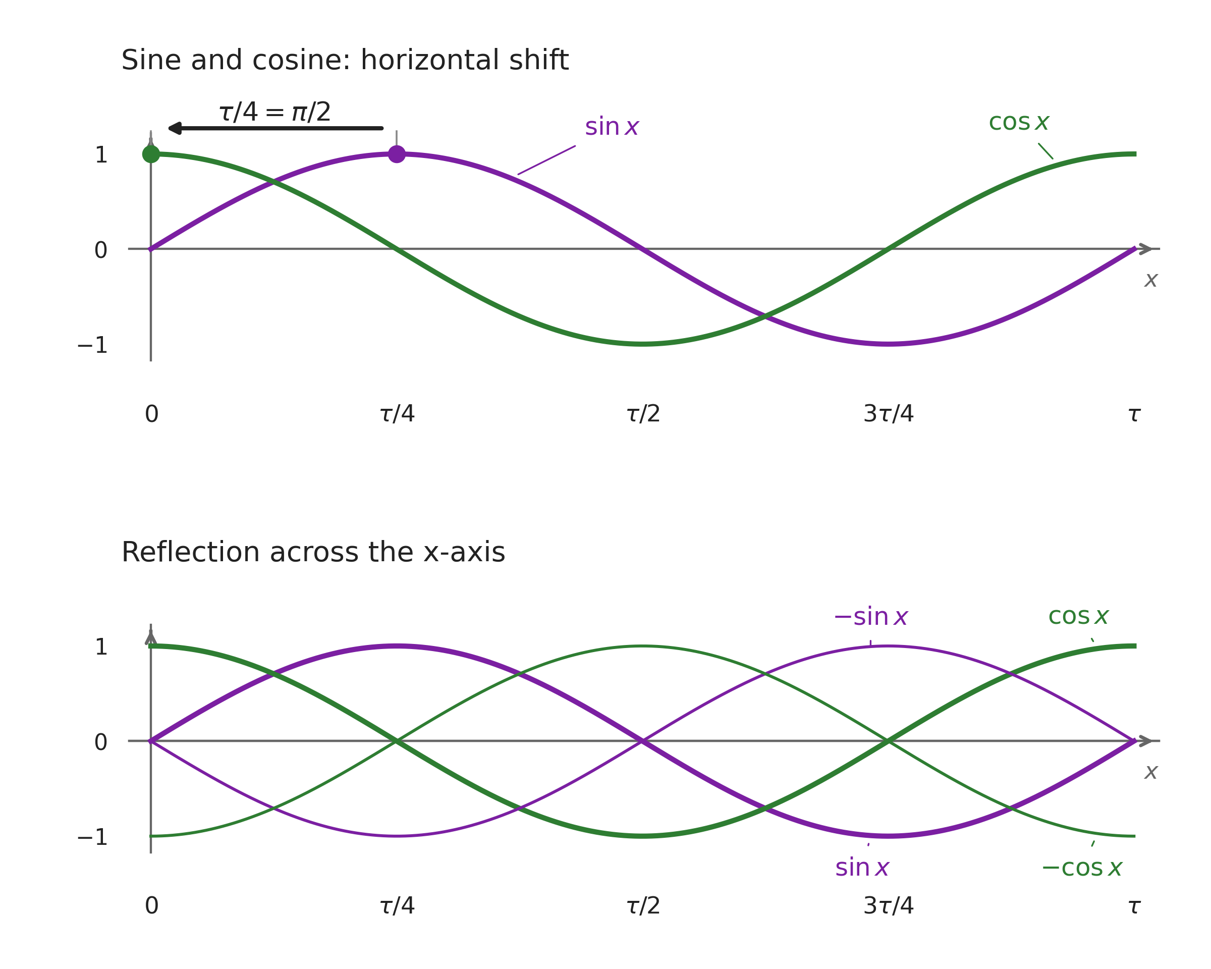
Notice that if we shift the sine wave to the left by \(\frac{\tau}{4}\), which is the same as \(\frac{\pi}{2}\) units, it matches perfectly with the cosine wave. This is a visual demonstration of how \(\sin\left( x + \frac{\tau}{4} \right) = \cos(x)\). In addition, multiplying the sine or cosine function by -1 shifts of the original graphs by \(\pi\) units.
To graph the tangent function, we must first remember that it is undefined at \(\frac{\tau}{4}\) radians, and any addition or subtraction of \(\frac{\tau}{2}\) from that. Graphing the function, we realize that when the x-values approach one of the points where it is undefined, the function blows up towards positive or negative infinity. The vertical lines through these x-values are known as vertical asymptotes, where a function zooms off towards infinity or negative infinity.
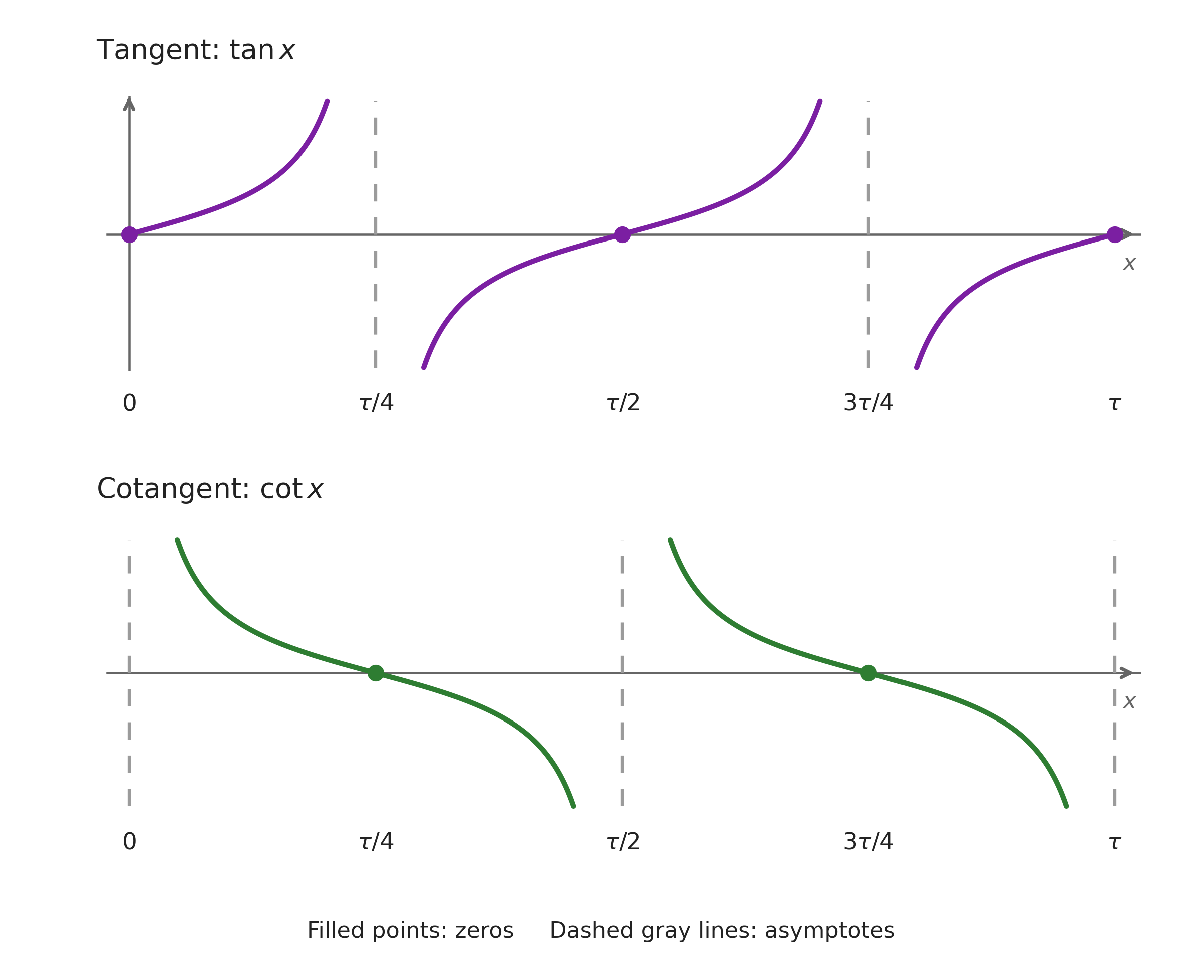
Focusing on the cotangent function, it blows up at the points where \(\tan(x) = 0\), because \(\frac{1}{0}\) is undefined. It is undefined at integer multiples of \(\tau/2\), where the sine denominator is zero. However, it has well-defined values at \(\frac{\tau}{4} + k\frac{\tau}{2}\), where \(k\) is any integer, because the cosine numerator is zero and the sine denominator is not. It is equal to zero at these points, and repeats every \(\tau/2\).
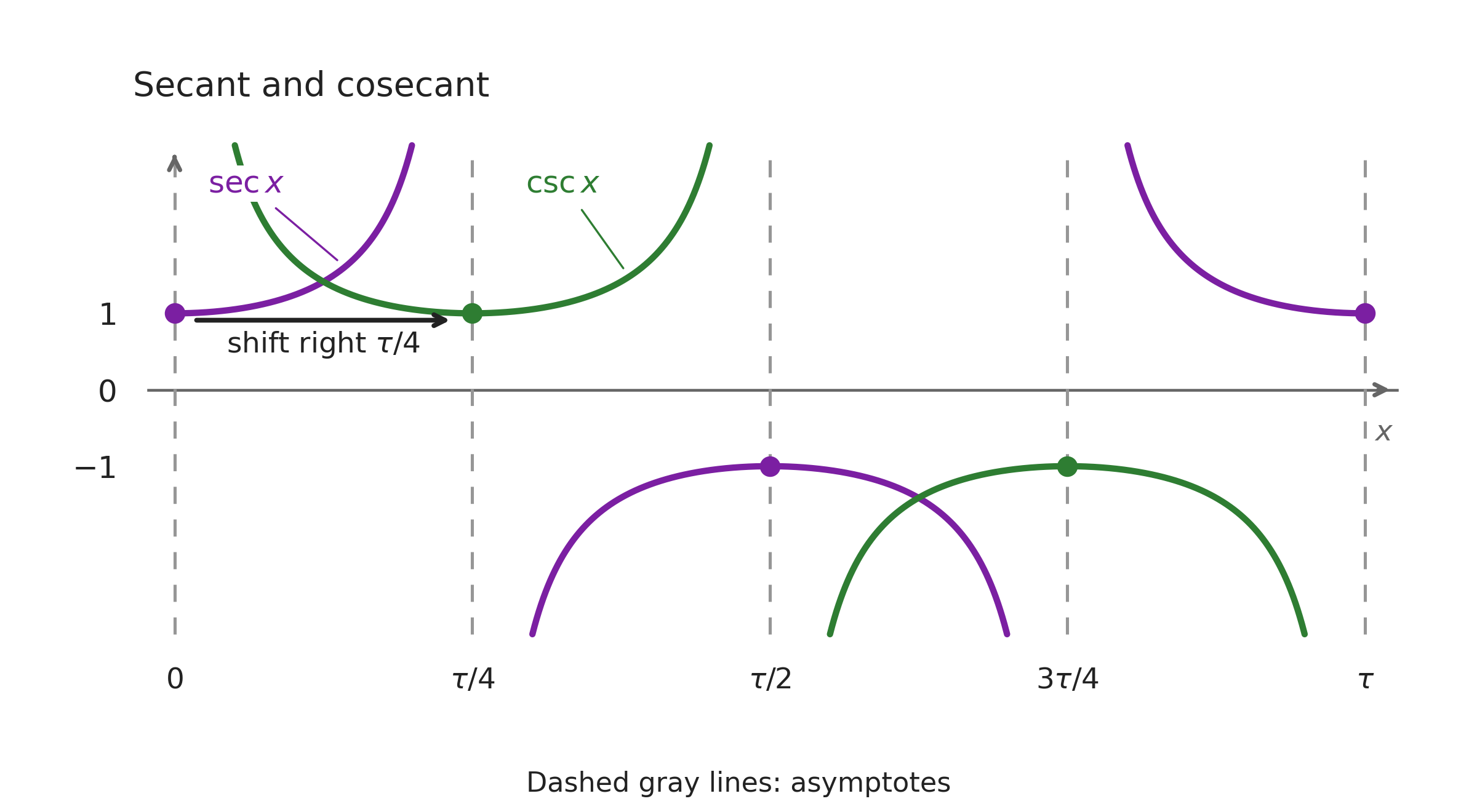
For the secant and cosecant functions, they will be undefined whenever their associated function is equal to zero. They will repeat every \(\tau\) units, and have a minimum of 1 on the positive side, because the sine/cosine maximum is 1. If a positive number is smaller than 1, then its reciprocal is larger than 1, so 1 is our minimum on the positive side. On the negative side, sine and cosine take values from -1 up to but not including zero, so their reciprocals are at most -1. Thus -1 is the maximum on the negative side, and the value with the smallest absolute value there. The graphs look like this:
Inverse Trigonometric Functions
We have seen how to find the \(x\) and \(y\) coordinates of a point on the unit circle using sine and cosine. But now the question is, what if we go in reverse? What if we already know one coordinate on the circle and we want to find the angle?
To do this, we can use the inverse trigonometric functions. The inverse cosine function, denoted by \(\cos^{- 1}(x)\) or \(\arccos(x)\), takes an x-coordinate on the unit circle and gives us the angle back. Because the maximum x-coordinate on a unit circle is one, and the minimum is -1, the function can only take inputs between -1 and 1. Likewise, the inverse sine function, written as \(\sin^{- 1}(y)\) or \(\arcsin(y)\), takes in the y-coordinate of a point and gives the angle. It is also restricted between -1 and 1.
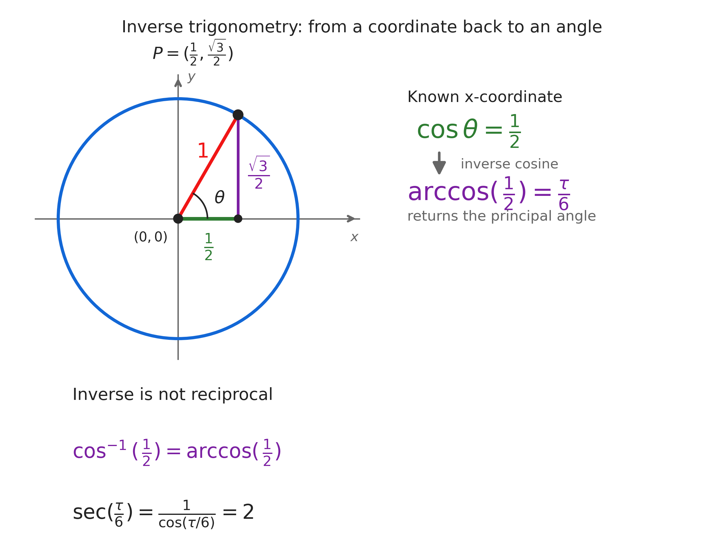
One important note is that a nonzero number to the power of -1, \(x^{- 1}\) for example, is the reciprocal of \(x\). However, the -1 power in the notation above does not mean reciprocal. It means inverse, which is not the same thing! As functions, \(\sin^{- 1} \neq csc\) and \(\cos^{- 1} \neq sec\). These functions are completely different! To avoid confusion, for the rest of the book I will be using the prefix “arc” to denote an inverse trigonometric function.
There are inverses of the rest of the trigonometric functions as well. They are denoted by \(\arctan(x)\), \(arcsec(x)\), \(arccsc(x)\), and \(arccot(x)\). These functions assume you already know the associated trig function of an angle, and give a principal angle back.
Looking at our diagram, the secant and cosecant of an angle can be anything except inside the circle, which is inside the range (-1,1). Therefore the \(arcsec(x)\) and \(arccsc(x)\) functions can handle any value except between (-1,1). The tangent and cotangent functions can output any number, so the \(\arctan(x)\) and \(arccot(x)\) can handle any number.
For an input in the domain of the inverse function, it is always true that \(\cos\left( \arccos{(x)} \right) = x\), and the same holds for the other inverse-function pairs.
However, there is a slight problem with trying to reverse the order of functions. The cosine function repeats every 2π (or \(\tau\)) units. So different angle values can lead to the same cosine value. But when you take the inverse cosine, it only gives back a value between 0 and \(\pi\), including both endpoints.
For example, if we take \(\cos(\frac{3}{2}\tau)\), this is the same as \(\cos(\frac{1}{2}\tau)\). We know that \(\cos\left( \frac{1}{2}\tau \right) = - 1\), so we need to find the \(\arccos( - 1)\). The function returns the principal angle \(\frac{1}{2}\tau\), rather than our original angle. The arccosine function “forgets” that we had added \(\tau\) to the angle.
If the original angle is already in the chosen principal range, the inverse does return that angle. To find all angles with the same cosine, we instead solve \(\cos\phi = cos\theta\). The solutions are \(\phi = \pm \theta + \tau k\), where \(k\) is any integer; the two signs account for reflection as well as full turns.
The same families apply to secant wherever it is defined. For sine and cosecant, the families are \(\phi = \theta + \tau k\) and \(\phi = \tau/2 - \theta + \tau k\), with undefined cosecant values excluded. The tangent and cotangent functions repeat every \(\pi\) units, instead of \(\tau\). So, the solutions of \(\tan\phi = tan\theta\) are \(\phi = \theta + \pi k\), and the same family works for cotangent wherever it is defined. These are sets of solutions, not the value of a principal inverse function.
What about the inverse trig functions? What do those graphs look like?
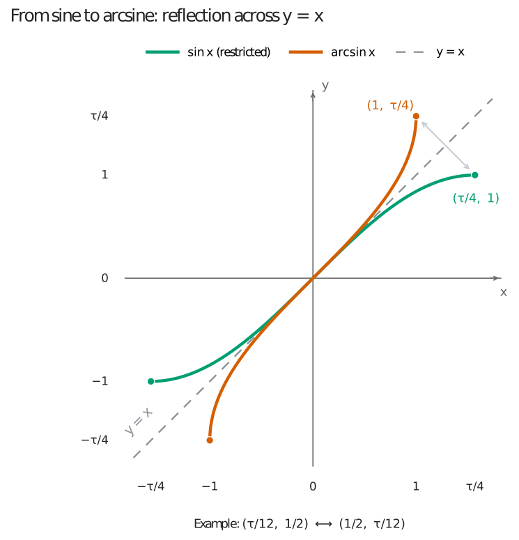
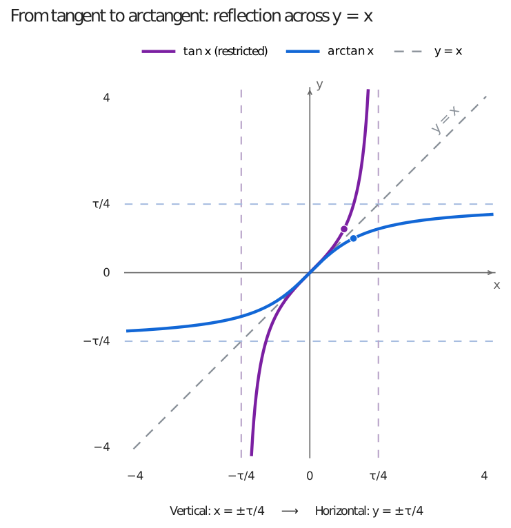
For arcsine and arccosine, their inputs are restricted between -1 and 1. There are many ways to think geometrically about inverse functions, but I have a relatively simple way to do it. To switch the original \(x\) and \(y\) values, we reflect the rotated graph over the line \(x = y\). This gives \(\left( \sin t,t \right)\), the inverse relation for sine.
However, we must remember that the arcsine function only outputs values between \(- \frac{\tau}{4}\) and \(\frac{\tau}{4}\), including both endpoints, so we restrict the graph to only that range. Our final graph for arcsine looks like:
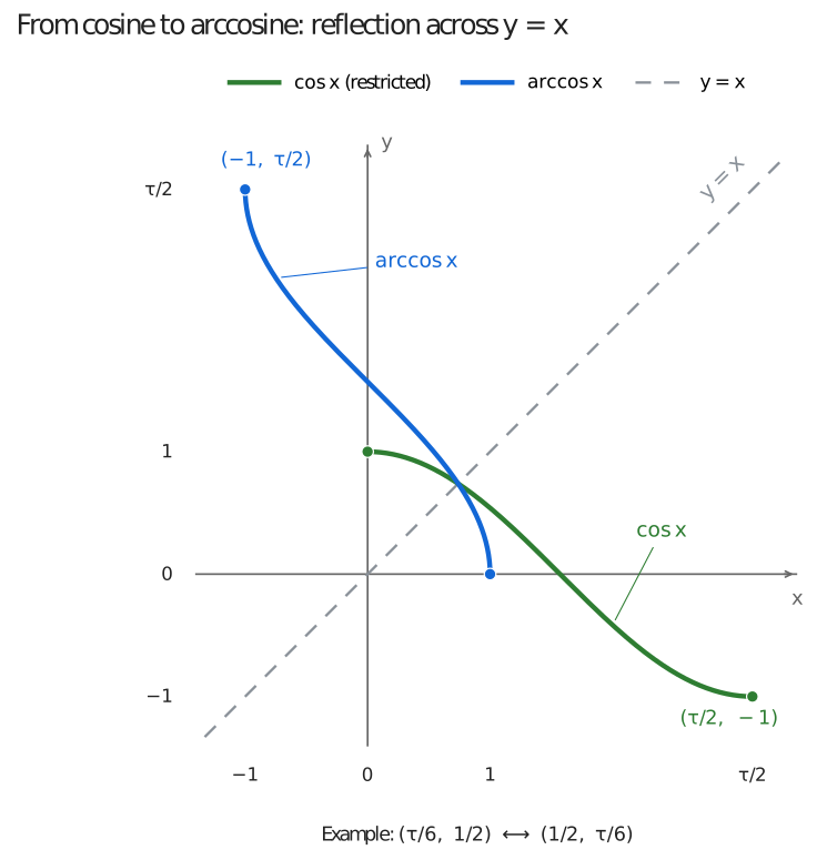
For arccosine, we restrict cosine to angles from 0 to \(\tau/2\), including both endpoints, before reflecting across \(y = x\). Its graph looks like this:
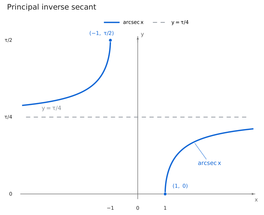
For inverse secant, the function can take in any value outside the open interval (-1,1), including -1 and 1. We use \(arcsec(x) = arccos(1/x)\), so it can only output angles between 0 and \(\frac{\tau}{2}\), including those endpoints but excluding \(\tau/4\). As \(x\) tends to positive or negative infinity, the output approaches \(\tau/4\) from below or above, respectively. Thus \(y = \tau/4\) is its horizontal (sideways) asymptote. The function looks like this:
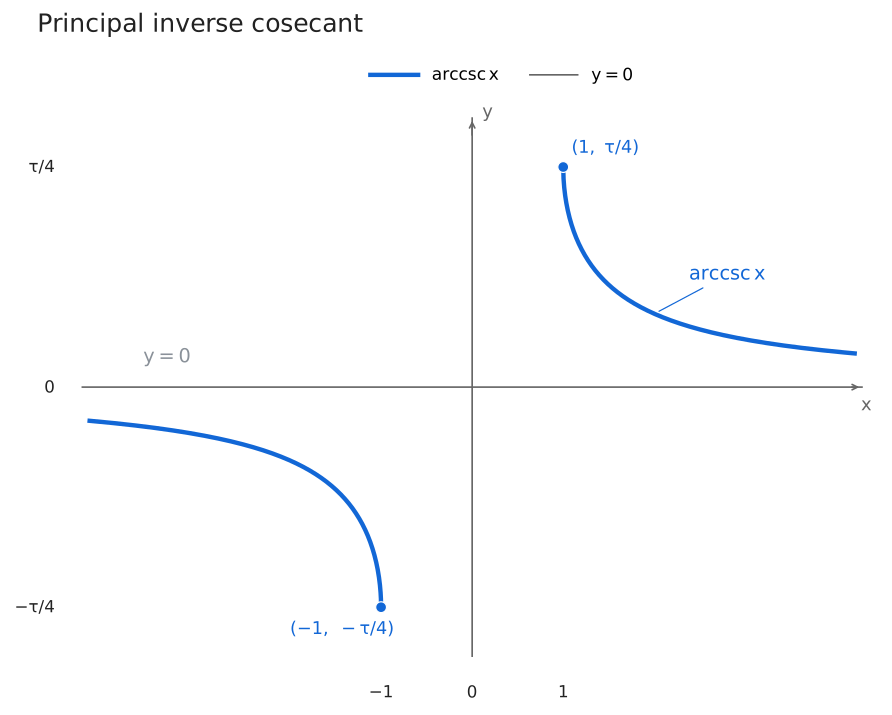
Similarly, we use \(arccsc(x) = arcsin(1/x)\) for \(x \leq - 1\ or\ x \geq 1\). Inverse cosecant has its output restricted between \(- \frac{\tau}{4}\) and \(\frac{\tau}{4}\). Both endpoints are included, but zero is excluded. Its graph is obtained by reflecting inverse secant across the x-axis and then shifting it upward by \(\tau/4\). Its horizontal asymptote is \(y = 0\).
For tangent and cotangent, we can use the same counterclockwise quarter-turn followed by reflection across the vertical axis to obtain their inverse relations, like this:
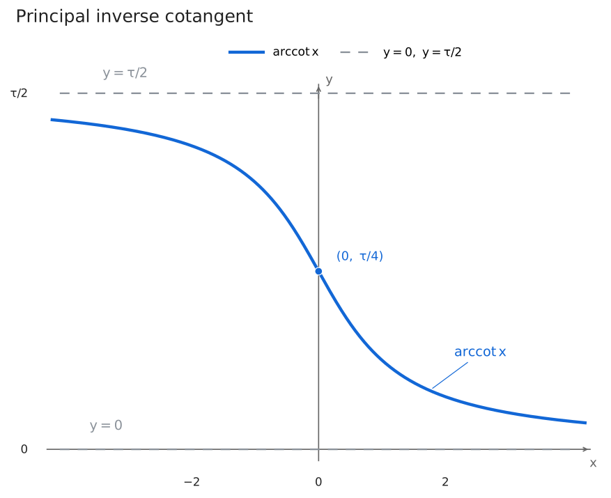
For arctangent, restrict the outputs to \(- \tau/4 < y < \tau/4\). For arccotangent, we will use \(0 < y < \tau/2\), where cotangent takes every real value exactly once. With this convention, \(arccot(x) = \tau/4 - arctan(x)\), including \(arccot(0) = \tau/4\). We end up with these final graphs:
Trigonometric Identities
Pythagorean Identities
These functions are connected in a variety of diverse ways, known as identities. We have already proved a few of them, such as \(\sin^{2}(\theta) + \cos^{2}(\theta) = 1\). From this identity, we can derive a similar one in terms of the tangent and secant functions. We want to find \(\tan^{2}(\theta) + 1\). Substituting for tangent and rewriting the one as a fraction,
\[\frac{\sin^{2}(\theta)}{\cos^{2}(\theta)} + \frac{\cos^{2}(\theta)}{\cos^{2}(\theta)}\]
But we already know that \(\sin^{2}(\theta) + \cos^{2}(\theta) = 1\), so the expression becomes
\[\frac{1}{\cos^{2}(\theta)} = \sec^{2}(\theta)\]
Our final identity is
\[\boxed{\tan^{2}(\theta) + 1 = \sec^{2}(\theta)}\]
Great!
We can also find \(\cot^{2}(\theta) + 1\) in much the same way. We can rewrite as
\[\frac{\cos^{2}(\theta)}{\sin^{2}(\theta)} + \frac{\sin^{2}(\theta)}{\sin^{2}(\theta)}\]
and using the same identity as before when combining fractions:
\[\frac{1}{\sin^{2}(\theta)}\]
Our final identity is similar to the one we previously derived:
\[\boxed{\cot^{2}(\theta) + 1 = \csc^{2}(\theta)}\]
The Law of Cosines
Before using the Law of Cosines, let’s see where it comes from. Suppose a triangle has sides \(a\), \(b\), and \(c\), with angle \(C\) between the sides of lengths \(a\) and \(b\). Place one vertex at \((0,0)\), the end of side \(b\) at \((b,0)\), and the last vertex at \(\left( a\cos C,a\sin C \right)\). This works because sine and cosine give the vertical and horizontal components of a segment.
The opposite side \(c\) joins the last two points. Using the distance formula and then squaring both sides, we have
\[c^{2} = \left( a\cos C - b \right)^{2} + \left( a\sin C \right)^{2}\]
Expanding the square gives
\[c^{2} = a^{2}\cos^{2}C - 2ab\cos C + b^{2} + a^{2}\sin^{2}C\]
The two terms containing \(a^{2}\) combine because \(\sin^{2}C + \cos^{2}C = 1\). Therefore
\[\boxed{c^{2} = a^{2} + b^{2} - 2ab\cos C}\]
This is the Law of Cosines. At \(C = 90^{\circ}\), the cosine term disappears and we get \(c^{2} = a^{2} + b^{2}\), the Pythagorean theorem.
Instead of being an unrelated new rule, the law extends that familiar theorem to triangles whose angles are not right angles. We can now use it to find the distance between two points on the unit circle, where both radii have length \(1\), and derive the cosine-difference identity that follows.
Sum and Difference Identities
So far, we have looked at functions and identities of a single variable. Sometimes it is helpful to be able to find out what the cosine or sine is of a sum or difference of two angles. Luckily, with a little bit of geometric interpretation and algebra we can get formulas for the cosine of two angles added or subtracted.
We first need to visualize what it looks like when we say \(\cos(A - B)\). In the picture, we have two angles, \(A\) and \(B\), and the middle angle, \(A - B\), is what we want to find the cosine of.
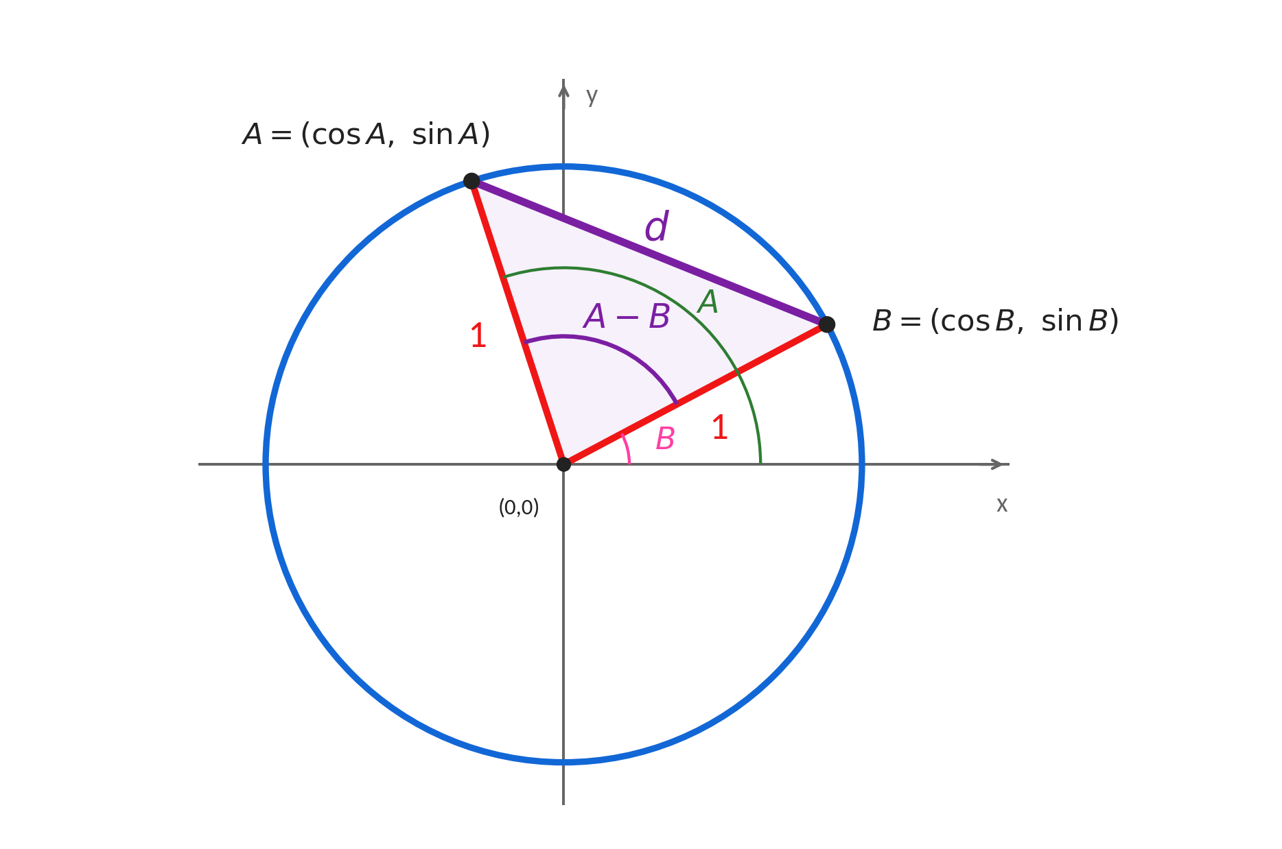
We can use the distance formula \(d = \sqrt{{(x_{2} - x_{1})}^{2} + {(y_{2} - y_{1})}^{2}}\) to find the distance from point \(A\) to point \(B\).
Plugging in for \(x\) and \(y\) using sine and cosine, we find
\[d = \sqrt{\left( \cos A - cosB \right)^{2} + \left( \sin A - sinB \right)^{2}}\]
On the other hand, we can use another trigonometric identity known as the law of cosines to find a different but equivalent expression for the distance. We have just proved this identity, which states that in any triangle, where \(a\), \(b\) and \(c\) are side lengths and \(C\) is the angle opposite side \(c\), \(a^{2} + b^{2} - 2abcos(C) = c^{2}\). If we take side \(c\) to be the distance we are looking for, then \(a\) and \(b\) are both 1 because of the radius of the unit circle. In our picture, angle \(C\) is simply \(A - B\). For other positions, the included angle may differ by a sign or full turns, but has the same cosine. Plugging in all our values, we find
\[d^{2} = 2 - 2\cos(A - B)\]
Squaring our first expression derived from the distance formula, we find that
\[d^{2} = \left( \cos(A) - \cos(B) \right)^{2} + {(\sin(A) - sin(B))}^{2}\]
Since these expressions are both equal to \(d^{2}\), they must be equal to each other. Therefore,
\[2 - 2\cos(A - B) = \left( \cos(A) - \cos(B) \right)^{2} + {(\sin(A) - sin(B))}^{2}\]
Expanding out the square terms, we find
\[2 - 2\cos(A - B) = \cos^{2}(A) - 2\cos(A)\cos(B) + \cos^{2}(B) + \sin^{2}(A) - 2\sin(A)\sin(B) + \sin^{2}(B)\]
We can simplify the square terms because \(\cos^{2}(A) + \sin^{2}(A) = 1\), and the same holds for \(B\), so:
\[2 - 2\cos(A - B) = 2 - 2\cos(A)\cos(B) - 2\sin(A)\sin(B)\]
We can divide through by -2, leaving
\[- 1 + cos(A - B) = - 1 + cos(A)\cos(B) + sin(A)\sin(B)\]
Finally, adding one to both sides gives us the cosine of difference identity:
\[\boxed{\cos(A - B) = \cos(A)\cos(B) + \sin(A)\sin(B)}\]
This is another amazing connection between the sine and cosine functions!
We can find the sum of angles just as easily by negating \(B\). The cosine function doesn’t change, but \(\sin( - B) = - \sin(B)\), so our sum identity is
\[\boxed{\cos(A + B) = \cos(A)\cos(B) - \sin(A)\sin(B)}\]
To find the sine of two angles, we must remember that \(\sin\left( 90^{{^\circ}} - \theta \right) = \cos(\theta)\). Therefore,
\[\sin(A - B) = \cos\left( 90^{{^\circ}} - (A - B) \right) = \cos(\left( 90^{{^\circ}} - A \right) + B)\]
Now we can treat \(90^{{^\circ}} - A\) as a new angle and use sum of angles:
\[\cos\left( 90^{O} - A \right)\cos(B) - \sin(90^{O} - A)\sin(B)\]
Converting the functions involving 90O-A back in terms of \(A\), we obtain
\[\boxed{\sin(A - B) = \sin(A)\cos(B) - \cos(A)\sin(B)}\]
As our final combination of angles identity, we can again replace \(B\) with -B to get the sum of angle formula for sine:
\[\boxed{\sin(A + B) = \sin(A)\cos(B) + \cos(A)sin(B)}\]
As special cases of our previously derived sums of angle identities, we can also consider the cosine and sine of twice an angle. To do this, simply set \(A = B\) in the above identities, and we can find that
\[\boxed{\cos(2A) = \cos^{2}(A) - \sin^{2}(A)}\]
One interesting fact is that if we add \(2\sin^{2}(A)\) to the right-hand side, it is equal to one, so the above equation can be rewritten as \(\cos(2A) = 1 - 2\sin^{2}(A)\). In the sine case
\[\boxed{\sin(2A) = 2\sin(A)\cos(A)}\]
The Chord Function
There are other, less commonly taught trigonometric functions that have historical significance. One of the most common that shows up in ancient times is the chord function. Just as modern trigonometry is based on the sine function, ancient Greek trigonometry was concerned with the lengths of chords.3
A chord is a line segment connecting two points on a circle. Chords are swept out by a specific angle, and the length of a chord given by an angle is the chord function, written as \(crd(\theta)\). In the context of the unit circle, the chord function is given by this line segment.
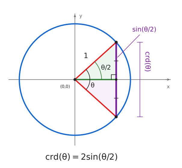
The chord function can be written in terms of the other trigonometric functions, using identities. Rotating the chord in Figure 4.22 counterclockwise by \(\theta/2\) puts its endpoints at the points \((1,0)\) and \((\cos(\theta),\sin(\theta))\), without changing its length. We can therefore use the distance formula. Plugging in, we get
\[crd(\theta) = \sqrt{\left( \cos(\theta) - 1 \right)^{2} + \sin^{2}(\theta)}\]
Expanding, we will get
\[crd(\theta) = \sqrt{\cos^{2}(\theta) - 2\cos(\theta) + 1 + \sin^{2}(\theta)}\]
Using the Pythagorean identity, we get an explicit formula for \(crd(\theta)\)
\[crd(\theta) = \sqrt{2 - 2\cos(\theta)}\]
Now, we can use half-angle formulas to get a different formula.
We can get the needed half-angle relation from the double-angle identity. Replacing its angle by \(\theta/2\) and rearranging gives
\[\cos\theta = 1 - 2\sin^{2}(\theta/2),\quad\quad\sin^{2}(\theta/2) = \frac{1 - cos\theta}{2}\]
Taking square roots introduces a sign. The Pythagorean identity gives the companion cosine formula:
\[\boxed{\sin(\theta/2) = \pm \sqrt{\frac{1 - cos\theta}{2}},\quad\quad\cos(\theta/2) = \pm \sqrt{\frac{1 + cos\theta}{2}}}\]
Choose each sign from the quadrant of \(\theta/2\); on an axis, the corresponding value may be zero.
Now substitute into our expression for the chord length:
\[crd(\theta) = \sqrt{2 - 2\cos\theta} = \sqrt{4\sin^{2}(\theta/2)} = 2\left| \sin(\theta/2) \right|\]
The absolute value matters because a length cannot be negative. If we take the angle between zero and one full turn, then its half lies between zero and a half turn, where sine is nonnegative. On that interval we can write the simpler formula
\[crd(\theta) = 2\sin(\theta/2),\quad\quad 0 \leq \theta \leq \tau\]
A half turn gives the diameter, with length two. A zero angle or a full turn brings both endpoints together and gives a chord of length zero.
Triple-Angle Identities
For our final exploration into trigonometric identities, we will consider what happens when we have the sine or cosine of three times an angle. This identity will be very useful in the next chapter. First, we consider \(\cos(3\theta) = \cos(2\theta + \theta)\). We can now expand using sum of angles as before:
\[\cos(2\theta)\cos(\theta) - sin(2\theta)sin(\theta)\]
Now we can expand out the \(\cos(2\theta)\) and \(\sin(2\theta)\) terms using the double-angle identities, yielding
\[\left( \cos^{2}(\theta) - \sin^{2}(\theta) \right)\cos(\theta) - 2\sin^{2}(\theta)\cos(\theta)\]
Multiplying out:
\[\cos^{3}(\theta) - \sin^{2}(\theta)\cos(\theta) - 2\sin^{2}(\theta)\cos(\theta)\]
Now we can rewrite \(\sin^{2}(\theta)\) as \(1 - \cos^{2}(\theta)\):
\[\cos^{3}(\theta) - \left( 1 - \cos^{2}(\theta) \right)\cos(\theta) - 2(1 - \cos^{2}(\theta))\cos(\theta)\]
Multiplying out again, we find:
\[\cos^{3}(\theta) - \cos(\theta) + \cos^{3}(\theta) - 2\cos(\theta) + 2\cos^{3}(\theta)\]
After combining like terms one more time, we can finally arrive at the triple-angle formula for cosine:
\[\boxed{\cos(3\theta) = 4\cos^{3}(\theta) - 3\cos(\theta)}\]
I will leave the triple-angle formula for sine as an exercise for the reader, but it uses mostly the same techniques as the derivation above. Your final answer should be equivalent to
\[\boxed{\sin(3\theta) = 3\sin(\theta) - 4\sin^{3}(\theta)}\]
Footnotes
Merriam-Webster, “Trigonometry,” Merriam-Webster.com Dictionary, accessed October 14, 2026, https://www.merriam-webster.com/dictionary/trigonometry.↩︎
Jeff Miller, “Cosine,” in “Earliest Known Uses of Some of the Words of Mathematics (C),” MacTutor History of Mathematics Archive, University of St Andrews, accessed October 14, 2026, https://mathshistory.st-andrews.ac.uk/Miller/mathword/c/.↩︎
J. J. O’Connor and E. F. Robertson, “Trigonometric Functions,” MacTutor History of Mathematics Archive, University of St Andrews, June 1996, https://mathshistory.st-andrews.ac.uk/HistTopics/Trigonometric_functions/.↩︎