Chapter 5½: The Exponential and Logarithmic Functions
An Interlude
In the last chapter, trigonometry gave us another way to solve cubic equations. Our next approach will use a different family of functions, but first we need to explore exponentials and logarithms.
The Constant \(\mathbf{e}\)
One of the most fundamental and important constants in all of mathematics is Euler’s number, denoted by \(e\). While its applications are complex and far reaching across all of math, it can be described using a simple puzzle.
Let’s say we have $1 that we want to invest in a savings account, and the bank is nice enough to offer 100% interest over a year. So, after 1 year, we have the initial $1 that we invested, and another dollar due to the 100% return, so $2 in total.
But, the bank offers us another option. Instead of taking 100% across the whole year, we can instead earn 50% interest over the first 6 months, then reinvest the money we got from there and earn 50% interest over the next 6 months. After the first 6 months, we would have $1.50 in our savings account. And, reinvesting this into our 50% return account, we would have $2.25 at the end of the year. Quite an improvement!
In technical terms, we compounded our money twice over the year, reinvesting our $1.50 into our account after the first 6 months. This is earning interest on our previously accrued interest.
But now, the bank offers us a third option. We can compound three times, once every 4 months, with an interest rate of \(33\frac{1}{3}\%\) to compensate. If we choose this option, we would have approximately $2.37 at the end of the year.
What if we have 25% interest, compounded every 3 months? Again, we would earn more money by the end, approximately $2.44.
Now the bank says we can choose to compound ANY number of times that we want, with the interest rate shifting to compensate. We saw that as the number of times we compounded increased, the amount of money we would receive also increased.
Could we earn infinite money off of this, or is there a limit?
Let’s construct a formula to show the amount of money we would receive at the end of the year. The interest rate is set at \(\frac{100}{n}\%\), where we compound \(n\) times. If the amount of money before a compounding period is \(m\), the amount of money after the compounding period is \(m\left( 1 + \frac{1}{n} \right)\), because \(m\) is added to the amount we get from interest payments. If the initial amount we have is \(m_{0} = 1\), and the amount after one compounding period is \(m_{1} = \left( 1 + \frac{1}{n} \right)\), then by repeatedly multiplying by \(1 + \frac{1}{n}\) for each compounding period, we get the formula
\[\boxed{A = \left( 1 + \frac{1}{n} \right)^{n}}\]
where \(A\) is the final amount of money at the end of the year.
We can observe two things about this formula. First, the number inside the parentheses is getting closer to one, which drives down the amount of money we would receive as our interest percentage is shrinking. But on the other hand, we have more times that we are compounding, and the exponent is rising. This makes the amount of money larger.
As we continue to increase \(n\), this tug-of-war continues, but the growth slows down.
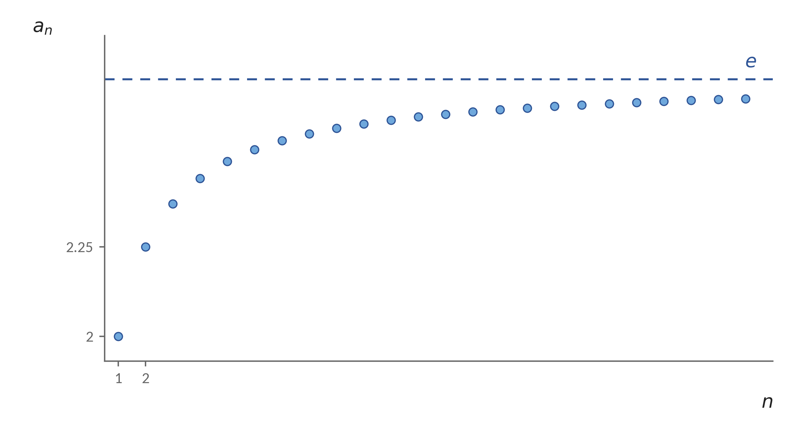
As we can see from the graph of this function, the extra gains from increasing the number of times we compound shrink, while the total money grows toward a number that is around \(2.72\). As the number of times we compound goes to infinity, the total money approaches the value of \(e\). Here are its first few digits: \(e \approx 2.71828182845\).
In the following chapters, we will see how \(e\) is connected to many areas of mathematics, especially complex numbers.
The Exponential Function
In the bank problem, \(e\) appeared as a single number, the limit of what our dollar could become. But we can use \(e\) in another way. Instead of keeping it as the answer to one calculation, we can make it the base of a function:
\[y = e^{x}\]
Now the exponent \(x\) is the input. What does changing \(x\) do to the graph?
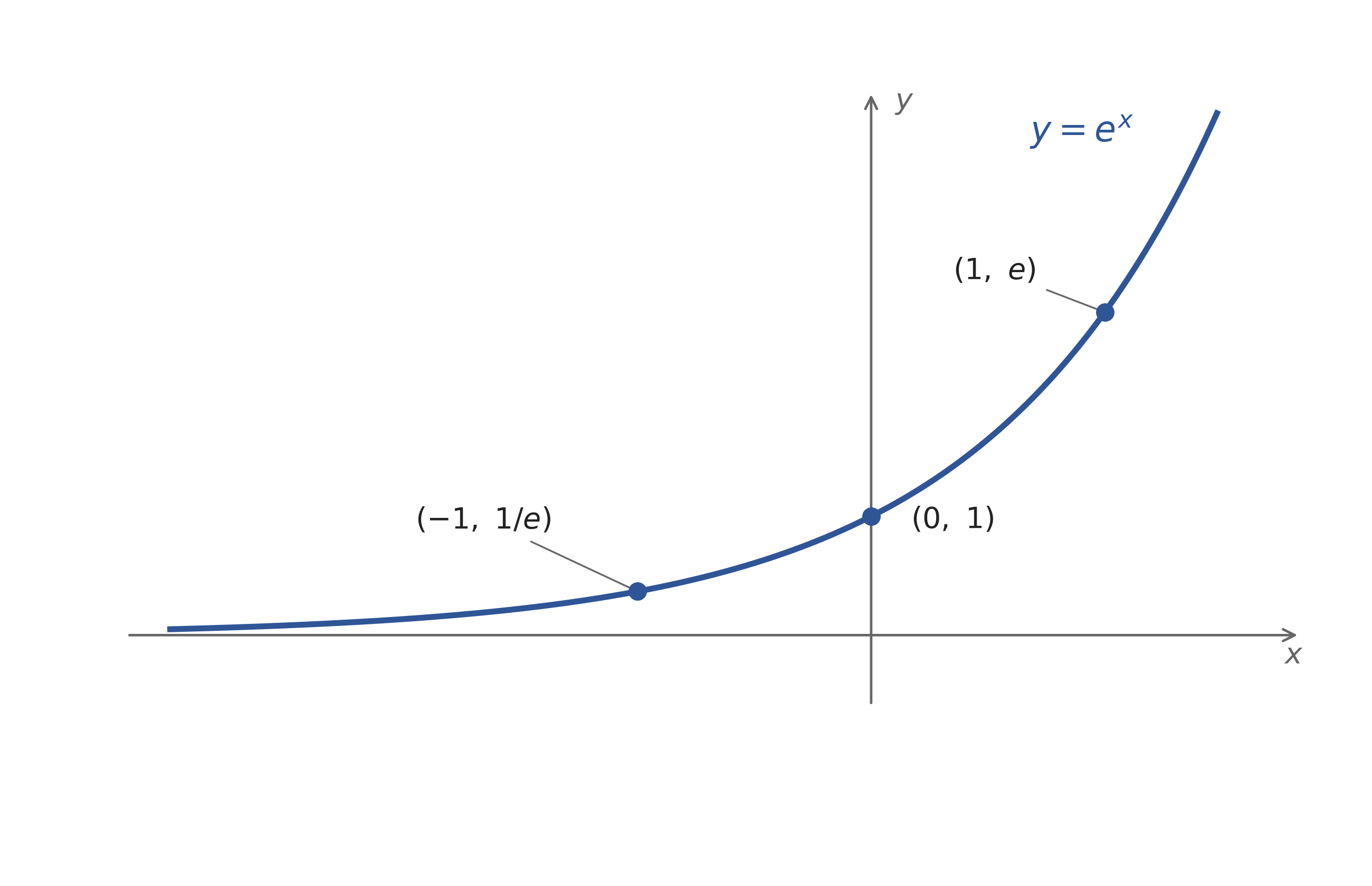
We can start with two values we already know. When \(x\) is zero, \(e^{0} = 1\), so the graph passes through \((0,1)\). When \(x\) is one, \(e^{1} = e\), giving us the point \((1,e)\). Because \(e\) is greater than one, the function rises as we move to the right. In fact, positive inputs give values greater than one.
But what happens when \(x\) is negative? At \(x = - 1\), we get \(e^{- 1} = 1/e\), a number between zero and one. All negative inputs give values between zero and one. As \(x\) gets more and more negative, \(e^{x}\) gets closer and closer to zero, but it never actually reaches zero. We call the x-axis a horizontal asymptote.
So this curve is always above the x-axis and increases from left to right. The same number we found through compounding interest now describes an entire function.
Applications of \(\mathbf{e}\)
\(e\) and the related function \(e^{x}\) are concepts that occur everywhere in mathematics and the physical world.
First, the function \(e^{x}\) expresses many instances of growth in the real world.
In the bank problem, the interest earned depended on how much money was already in the account. A bigger balance earned more interest at the same rate. Now here's something special about our new function, \(y = e^{x}\): its instantaneous rate of change with respect to \(x\) is equal to the value of the function itself.
When the input is \(1\), \(y = e\) and its rate is \(e\). When the input is \(2\), \(y = e^{2}\) and its rate is \(e^{2}\). The function grows, and the rate at which it grows increases right along with it.
We would need calculus to prove this, which we won't go into here. But it helps explain why \(e\) appears so often when we study growth.
Logarithms
So far, we've used exponents to find values. But what if we know the value and need to find the exponent? Suppose
\[10^{x} = 1000.\]
Well, \(10^{3} = 1000\), so \(x = 3\). This is an exponential calculation in reverse, and we have a name for it: a logarithm. We write
\[\log_{10}(1000) = 3.\]
The little \(10\) tells us which base we're using. For real logarithms, we need \(b>0\), \(b\ne1\), and \(y>0\). In general,
\[\boxed{\log_{b}(y) = x\quad\quad \Leftrightarrow \quad\quad b^{x} = y}\]
This can get confusing with roots/radicals, so the way I like to remember it is “radicals take the top off, logarithms take the bottom out”. This is because roots output the base, and take the exponent “top” off, while logarithms output the exponent given the base “bottom out”.
We can also choose \(e\) as our base. This is called the natural logarithm, written \(\ln\). So,
\(\ln(y) = x\) means \(e^{x} = y\)
For instance, \(\ln(1) = 0\) and \(\ln(e) = 1\).
Reversing the exponential switches the input and output. Since \(e^{0} = 1\), the point \((0,1)\) lies on the graph of \(y = e^{x}\).
Reversing those coordinates gives \((1,0)\) on the graph of \(y = lnx\). The same switch works for every point, so the two graphs are reflections of each other across the line \(y = x\).
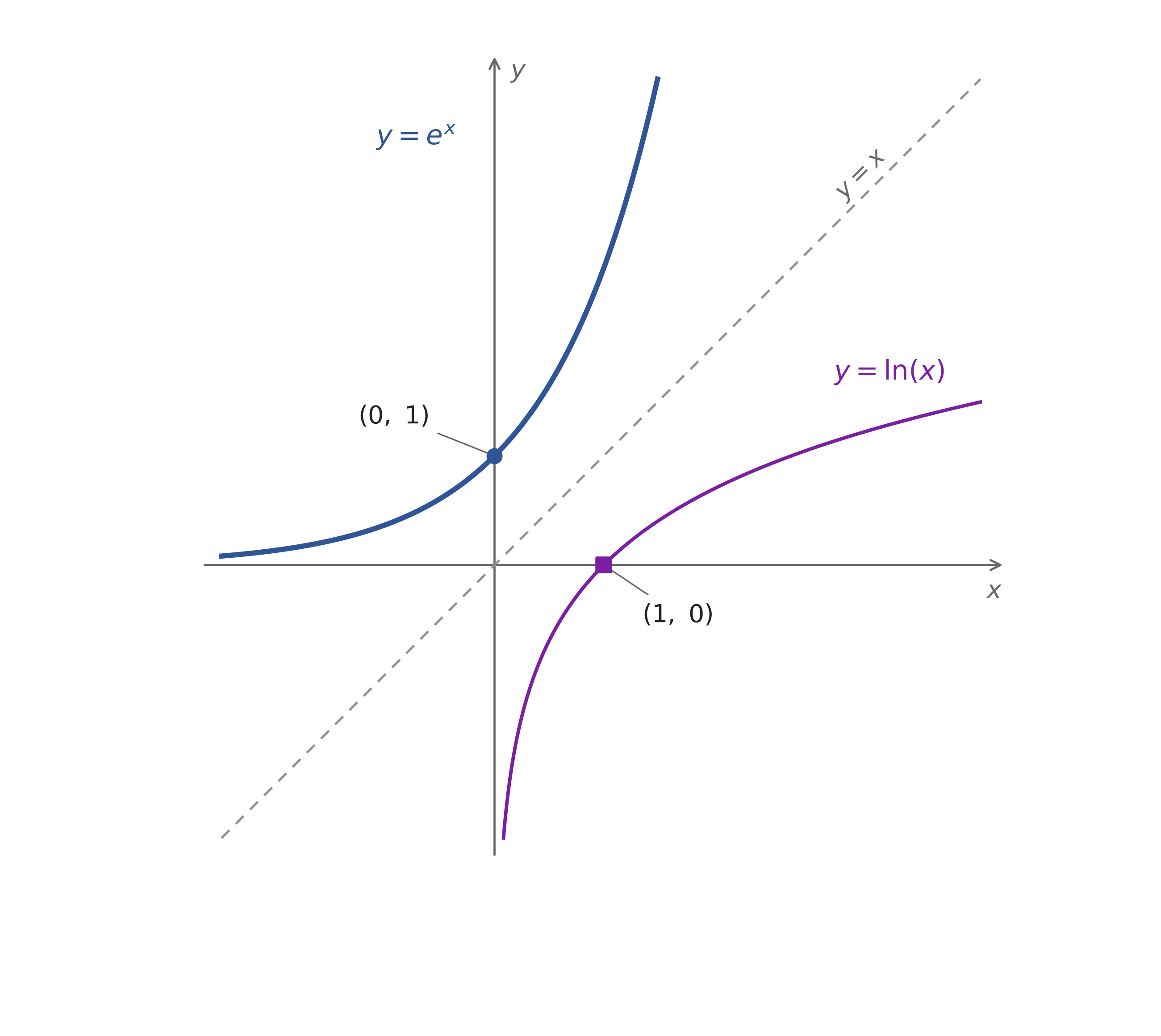
This also explains the restriction on the logarithm’s input. The exponential only gives positive outputs, so the real natural logarithm only accepts positive inputs. In symbols, the two directions are
\[\boxed{\ln\left( e^{x} \right) = x\quad\left( x\mathbb{\in R} \right),\quad\quad e^{\ln x} = x\quad(x > 0)}\]
The exponent laws give us rules for logarithms too. If \(u = b^{A}\) and \(v = b^{B}\), multiplying gives \(uv = b^{A + B}\). Taking the base-\(b\) logarithm therefore gives
\[\log_{b}(uv) = \log_{b}u + \log_{b}v.\]
Multiplication inside the logarithm has become addition outside it. For example,
\[\log_{10}(100 \cdot 1000) = \log_{10}100 + \log_{10}1000 = 2 + 3 = 5.\]
The product is \(100000 = 10^{5}\), which checks the result directly.
In fact, this property was used for hundreds of years to calculate complicated multiplications. Instead of multiplying all of the numbers together, you would look up the logs of both numbers in a book, then add them together. Even the slide rule, a fantastic mechanical calculator used before modern electronics, employs the logarithmic scale.1
Dividing powers subtracts their exponents, and raising a power to another power multiplies the exponents. The corresponding logarithm rules are
\[\log_{b}\left( \frac{u}{v} \right) = \log_{b}u - \log_{b}v,\quad\quad\log_{b}\left( u^{r} \right) = r\log_{b}u.\]
When \(u,v > 0\), \(b > 0\), \(b \neq 1\), and \(r\) is real. These rules also work for \(\ln\), since it is just the logarithm with base \(e\).
We can even calculate a logarithm in another base using natural logarithms. If \(x = \log_{b}u\), then \(b^{x} = u\). Taking natural logarithms and using the power rule gives \(x\ln b = lnu\), so
\[\log_{b}u = \frac{\ln u}{\ln b}.\]
We've now learned how to work forward with exponentials and backward with logarithms. But we're not finished with \(e\). In the next chapter, we'll add and subtract \(e^{x}\) and its reciprocal \(e^{- x}\). Why would that have anything to do with geometry? The result will take us to a hyperbola. We'll return to logarithms again when we extend these ideas to complex numbers.
Footnotes
1Whipple Museum of the History of Science, University of Cambridge, “Tables,” https://www.whipplemuseum.cam.ac.uk/explore-whipple-collections/calculating-devices/tables; Smithsonian Institution, National Museum of American History, “Linear Slide Rules,” https://www.si.edu/spotlight/slide-rules/linear-slide-rules.↩︎