Chapter 8: Euler’s Formula and Complex Logarithms
Euler’s Formula and Identity
In Chapter 5½, we studied exponentials and logarithms using real numbers. Then, in Chapter 7, we described complex numbers by their magnitudes and angles. We have also seen that complex numbers supply the roots of polynomial equations, even when the real numbers fall short.
So, what happens if we allow the exponential function to take imaginary inputs? As we will see, this brings the geometry of the circle into the same formula as exponentials. To understand why, we need infinite series.
Infinite Series
An infinite series is the sum of infinitely many terms. When its partial sums approach a specific value, the series converges. They are often used by computers to approximate values of roots, trigonometric functions, and other functions. In fact, the approximations provided in this book were derived by my computer, which used infinite series approximations.
One more thing that is essential to know about infinite series is that they often use the factorial function. The factorial function represents how many ways a number of objects can be arranged, denoted by \(n!\). If I have four objects, labeled 1-4, the number of ways you can order them is \(4!\). To compute what \(4!\) is, we consider all the possible positions of objects. For the first object, you have four choices of where to put it. For the second, you only have three choices as one spot in the order is already filled. Likewise, for the third object, you only have two options, and for the last one you only have one choice. So the total number of arrangements of four objects is \(4*3*2*1 = 24\).
This can be extended to the factorial of any positive integer, so to take a factorial of a number means multiplying that number by all positive integers below it.
One of the great properties of the number \(e\) is that it can be approximated very accurately by an infinite sum of fractions.
\[e = 1 + \frac{1}{1!} + \frac{1}{2!} + \frac{1}{3!} + \frac{1}{4!}\ldots\]
This formula can be extended to represent \(e\) to the power of any number, like this:
\[e^{x} = 1 + x + \frac{x^{2}}{2!} + \frac{x^{3}}{3!}\ldots\]
Similarly, using some calculus, we can get infinite series for the sine and cosine functions. However, in these series, the fractions are repeatedly added and subtracted. Each is known as an alternating series, because the signs of successive terms alternate. These formulas are what your computer uses to calculate trig functions!
Note that these formulas only work when the angles are in radians.
\[\sin(x) = x - \frac{x^{3}}{3!} + \frac{x^{5}}{5!} - \frac{x^{7}}{7!}\ldots\]
\[\cos(x) = 1 - \frac{x^{2}}{2!} + \frac{x^{4}}{4!} - \frac{x^{6}}{6!}\ldots\]
Extension to the Complex Numbers
In the mid-1700s, the great mathematician Leonhard Euler had an amazing insight.1 We know the formula works when we plug in a real number. What happens if we plug in an imaginary number? While it is practically impossible to visualize “multiplying \(e\) by itself \(i\) times”, we can plug into the formula and see what happens. If we try to find what \(e^{ix}\) looks like, we find that
\[e^{ix} = 1 + ix - \frac{x^{2}}{2!} + \frac{{ix}^{3}}{3!} + \frac{x^{4}}{4!}\ldots\]
The powers of \(i\) repeat in a cycle: \(i^{2} = - 1\), \(i^{3} = - i\), and \(i^{4} = 1\).
This makes the even-powered terms alternate between positive and negative real terms, while every odd-powered term contains a factor of \(i\). Once we gather the two groups separately, we can recognize the series for cosine and sine.
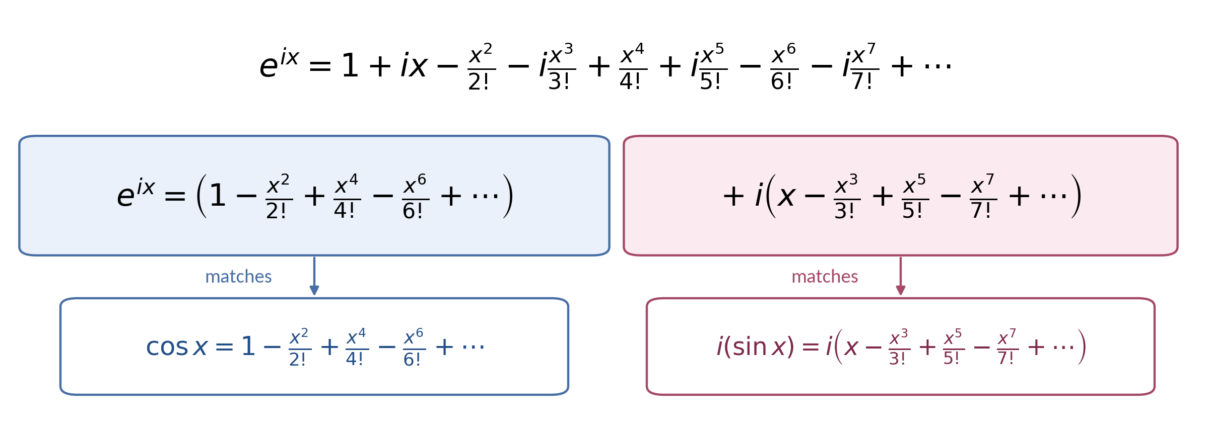
This looks familiar. In fact, if we separate all the even \(x\) powers from odd \(x\) powers, we find \(e^{ix} = 1 - \frac{x^{2}}{2!} + \frac{x^{4}}{4!}\ldots + ix - \frac{ix^{3}}{3!} + \frac{ix^{5}}{5!}\ldots\). The first half perfectly resembles our infinite formula for cosine, and the second half is our infinite series for sine, with a factor of \(i\) attached to all of the terms.
Therefore, we derive that
\[\boxed{e^{ix} = \cos(x) + i\sin(x)}\]
From this important identity, we can derive one of the most profound equations in all of mathematics.
Plugging in \(\pi\) for \(x\) (we are working in radians), we find \(\cos(\pi) = - 1\) and \(\sin(\pi) = 0\). So \(e^{i\pi} = - 1\). Adding 1 to both sides, our final equation is
\[\boxed{{\ e}^{i\pi} + 1 = 0\ }\]
This equation unites the five most important constants in mathematics, \(e\), \(\pi\), \(i\), \(1\) and \(0\), into a single equation, and contains the three basic arithmetic operations of addition, multiplication and exponentiation exactly once.
Many have considered it to be the most beautiful equation in all of mathematics, and entire books have been written focusing on this equation.2 If you remember only one thing from this book, it should be this identity.
Complex Numbers in Exponential Form
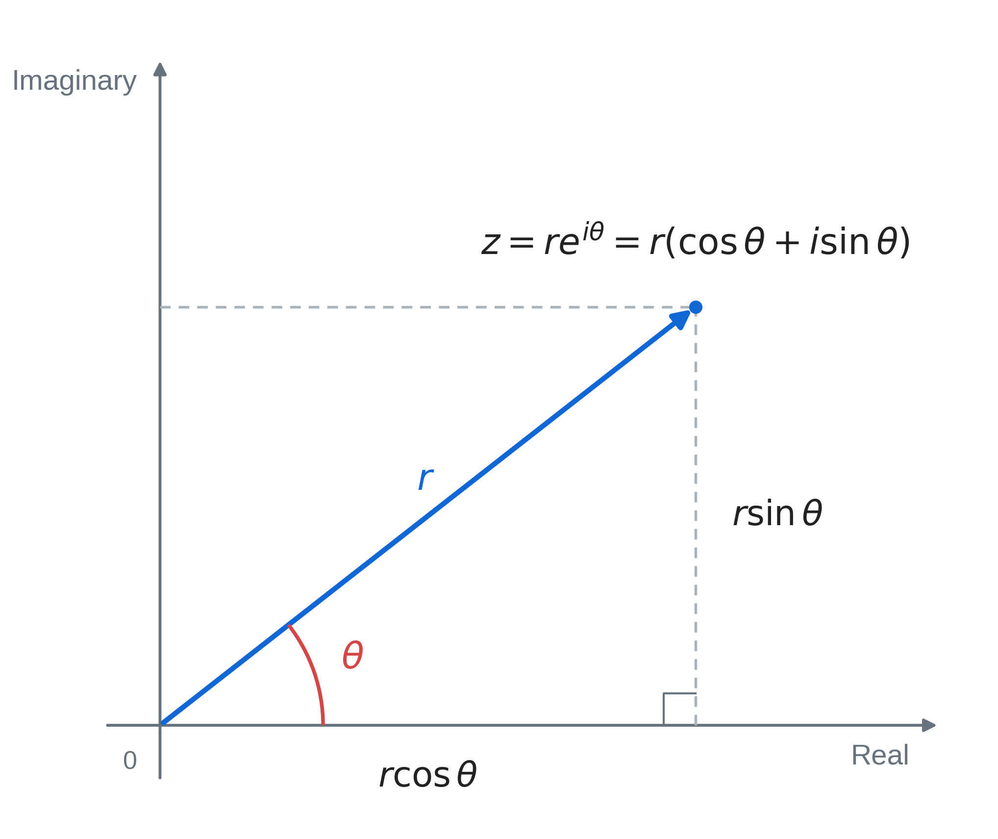
Furthermore, the identity \(e^{ix} = \cos(x) + i\sin(x)\) provides a nice way to represent polar coordinates numerically. Previously, polar coordinates were useful but didn’t have an actual numeric representation. But now, we can realize that our conversion formula for a magnitude of 1 matches up perfectly with the right side!
So, \(x\) in the identity really represents the angle of the complex number in polar coordinates!! We can extend this to complex numbers of all magnitudes by multiplying our identity by \(r\), our magnitude.
\[\boxed{re^{i\theta} = r\cos(\theta) + risin(\theta)}\]
This formula allows us to express polar coordinates as an exponent of \(e\).
Multiplication, Division, and Integer Powers
This allows us to reinterpret complex number multiplication and division. Previously, we have shown that multiplying complex numbers is equivalent to multiplying their magnitudes and adding their angles through trigonometric identities.
However, this compact representation of polar form provides a much faster proof. If we take two complex numbers, \(a\) and \(b\), and multiply them together, this is equivalent to
\[\left( r_{a}e^{i\theta_{a}} \right)\left( r_{b}{\ e}^{i\theta_{b}} \right) = \left( r_{a}\ r_{b} \right){\ e}^{i\theta_{a\ }}e^{i\theta_{b}}\]
Using laws of exponents, we can combine our two exponential terms, leaving
\[\left( r_{a}{\ r}_{b} \right)\ e^{i(\theta_{a} + \theta_{b})}\]
This proves our above identity in only three lines!
What about division? Dividing the exponential terms subtracts their exponents, so for complex numbers we divide their magnitudes and subtract their angles.
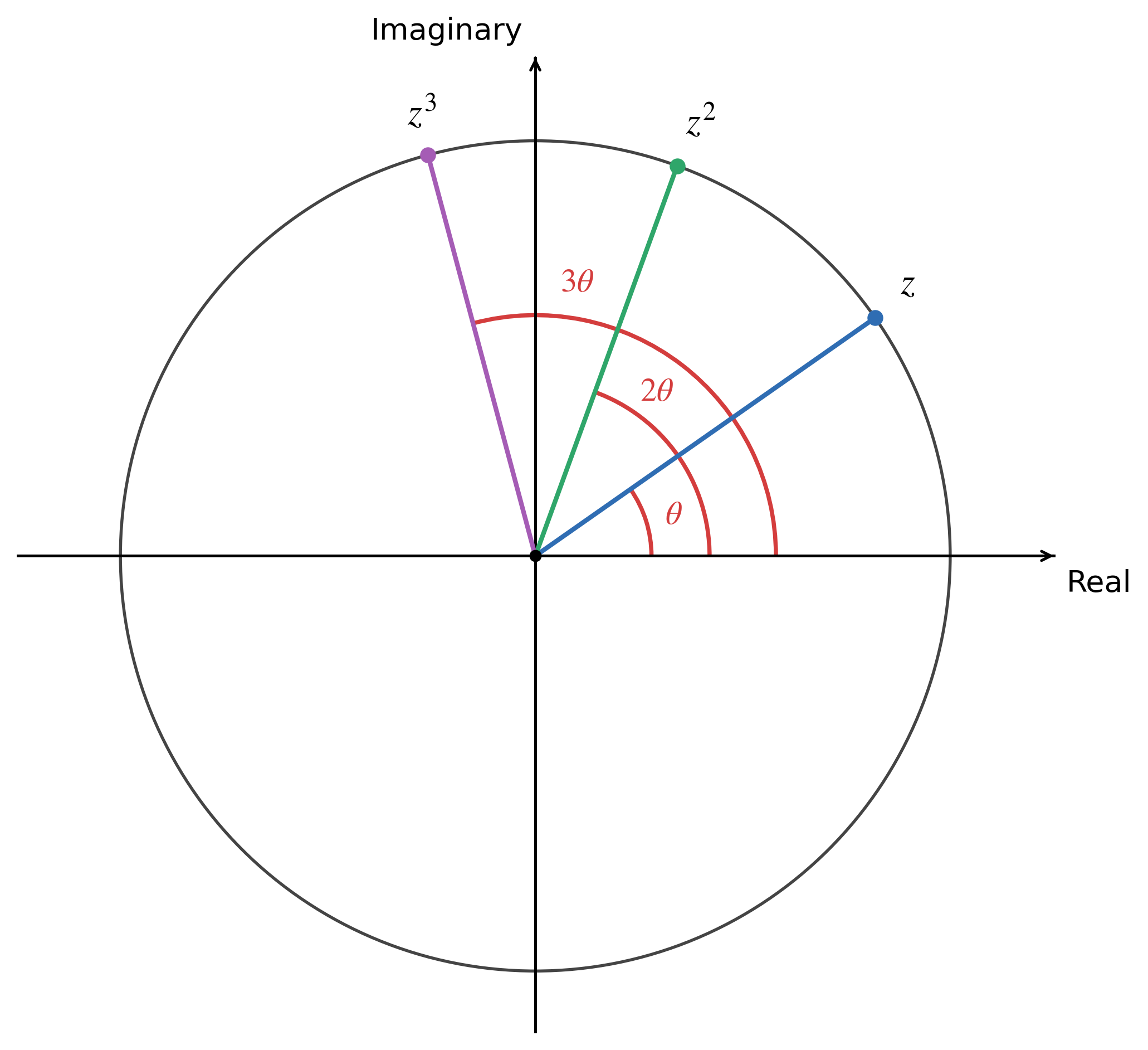
What happens if we multiply the same complex number by itself several times? Its magnitude is raised to that power, while its angle is multiplied by the power.
Negative integer powers take reciprocals, so the same rule works for them. The zeroth power of a nonzero number is 1. As before, adding a full turn does not change the number.
Connections to the Roots of Unity
This formula has a deep connection to the roots of unity. Recall that, for \(n \geq 3\), the set of nth roots of unity forms a regular polygon with \(n\) sides. This means that the angles are multiples of \(\frac{\tau}{n}\), and therefore the nth roots of unity can be expressed as \(e^{\frac{\tau}{n}i}\), \(e^{\frac{2\tau}{n}i}\)… up to \(n\).
Furthermore, we can easily prove that the integer powers of a root of unity are other roots of unity. For example, by laws of exponents, we can show that the first cube root of unity, when squared, is equal to the second cube root of unity. It can be written as \(\left( e^{\frac{\tau}{3}i} \right)^{2}\), so by laws of exponents this is \(e^{\frac{2\tau}{3}i}\), the second cube root of unity.
In general, this is true because raising a root of unity to an integer power multiplies its exponent by that integer, producing another root of unity. This is the precise reason why the exponential formula is so useful, as it allows us to express the geometry of complex numbers in terms of the familiar algebra of exponentials.
Complex Logarithms
An idea that comes up a lot in complex analysis is known as analytic continuation. This sounds scary, but it means extending an analytic function beyond its original domain while preserving its analytic behavior. We have already extended square roots to negative numbers via the definition of \(i\), and using Euler’s identity, we can extend the logarithm function to negatives and beyond.
We introduced real logarithms and their basic rules in Chapter 5½. There, the logarithm of a positive number undoes exponentiation, and multiplying positive numbers turns into addition of their logarithms. But real logarithms do not accept negative inputs. Now that the exponential function also works with complex numbers, we can ask what a logarithm of a negative or complex number should mean. The answer has a surprise: there can be infinitely many values.
Logarithms of Negative Numbers
Real logarithms cannot take negative inputs, but we can ask which complex numbers \(w\) satisfy \(e^{w} = - 1\).
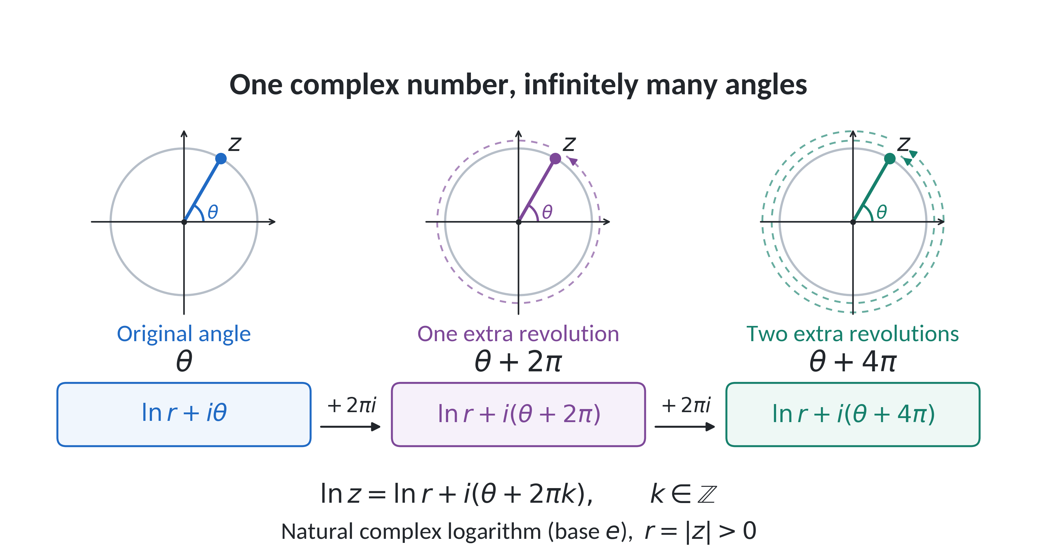
Euler’s formula tells us \(e^{i\pi} = - 1\). Yet an angle can increase by a whole turn without changing the exponential, so the complete set of answers is
\[w = i(\pi + 2\pi k),\quad where\ k\ is\ an\ integer\]
This is our first example of a multivalued complex logarithm: every integer \(k\) gives another value. Choosing \(k = 0\) produces the principal value \(Log( - 1) = i\pi\). For a negative real number \(- n\), where \(n > 0\), its magnitude contributes the ordinary real logarithm \(\ln n\), so the full family is
\[\log( - n) = lnn + i(\pi + 2\pi k),\ \ \ \ \quad where\ k\ is\ an\ integer\]
For example, \(\log( - 2)\) has values \(\ln 2 + i\pi\), \(\ln 2 + 3i\pi\), and infinitely many more. The important point is that we are solving an exponential equation, not assuming that all the familiar product rules for real logarithms carry over unchanged to one selected complex branch. Figure 8.4 shows why the different answers correspond to different descriptions of the same angle.
Logarithms of Complex Numbers
Now that we have found the logarithm of a negative number, can we find the natural logarithm of a complex number? For example, what is \(\ln(1 + 2i)\)?
To compute this, we convert to polar form and write this in exponential form. The magnitude of \(1 + 2i\) is \(\sqrt{1^{2} + 2^{2}} = \sqrt{5}\).
Our angle is \(\arctan\left( \frac{2}{1} \right) = \arctan(2)\)
Therefore, \(1 + 2i = \sqrt{5}\ e^{iarctan(2)}\)
Now we can take the natural logarithm:
\[\text{Log}\left( \sqrt{5}*e^{iarctan(2)} \right) = \ln\left( \sqrt{5} \right) + \text{Log}(e^{iarctan(2)})\]
Simplifying and adding on \(2\pi ki\) to account for all solutions, we arrive at
\[\ln(1 + 2i) = \frac{1}{2}\ln(5) + i\arctan(2) + 2\pi ik\]
Assuming \(k = 0\), we can approximate its logarithm as \(\text{Log}(1 + 2i) \approx 0.8047 + 1.1071i\).
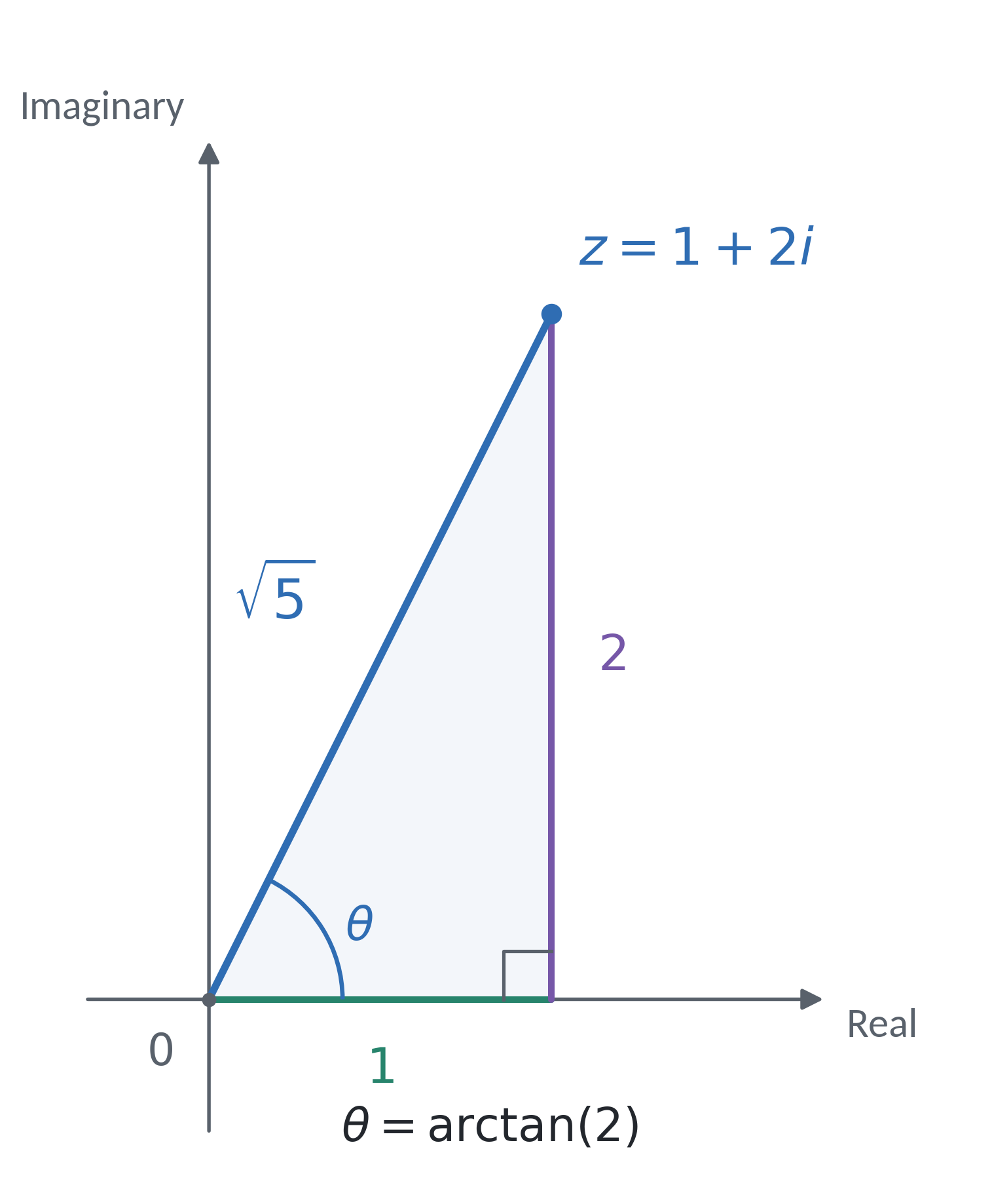
But what does the natural logarithm of a complex number really mean? Let’s look at what we did to find the logarithm. We found the magnitude of the number, then took the natural logarithm. This is our real part. Our imaginary part is our angle.
So, the complex logarithm outputs a complex number with real part \(\ln(r)\) and imaginary part \(\theta\), or \(\ln(r) + i\theta\). This natural logarithm can again be extended to any positive base other than 1 by the logarithmic base change formula.
The Principal Logarithm
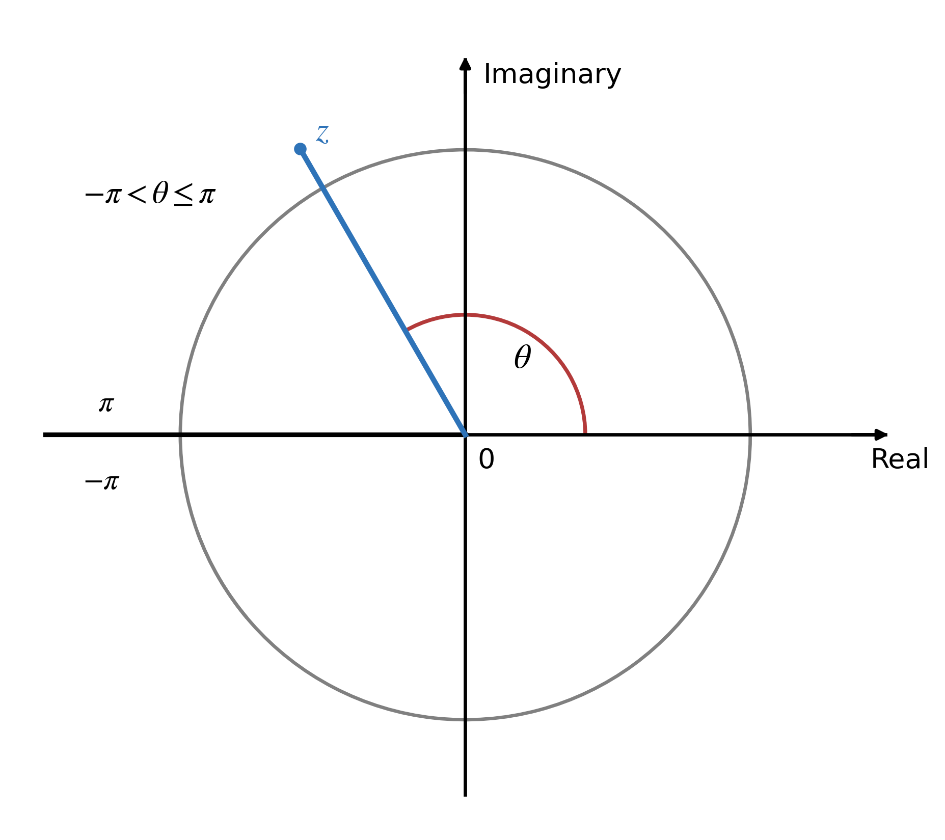
The angle of a complex number can change by a full turn without changing the number. To choose one logarithm value, we use the principal argument, \(- \pi\ < \ \text{Arg}\ z\ \leq \ \pi\), and write
\[\boxed{\text{Log}\ z\ = \ \text{ln}|z|\ + \ i\ \text{Arg}\ z}\]
All logarithm values are \(\text{Log}\ z\ + \ 2\pi ik\), where \(k\) is any integer. Our formulas written as \(\text{ln}\ z\ = \ \cdots\ + \ 2\pi ik\) describe that whole family. We keep \(\text{ln}\ r\) for the ordinary real logarithm when \(r\ > \ 0\). This chosen branch is not continuous across the negative real axis.
A Connection to Hyperbolic Functions
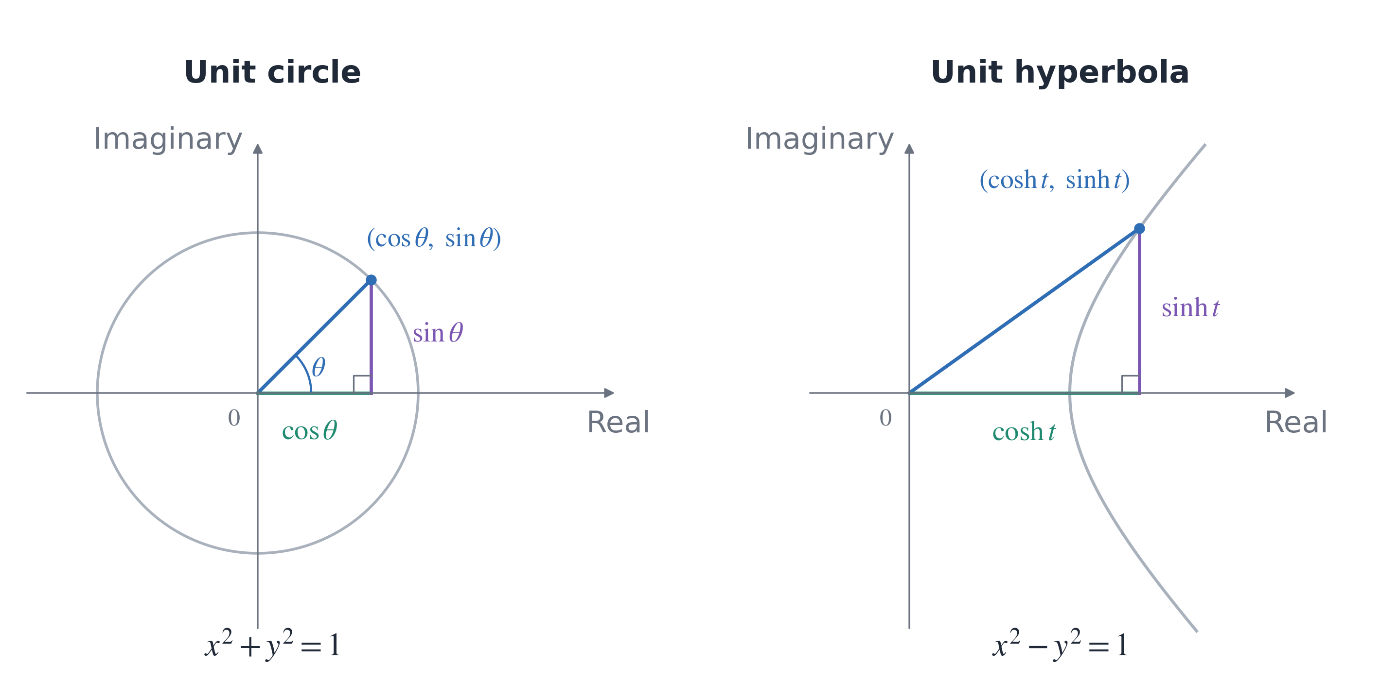
We can now write points on a circle using exponentials. But exponentials also appeared in our formulas for the hyperbola. How are those two pictures connected? Adding and subtracting Euler’s formula at \(t\) and \(- t\) gives, for real \(t\),
\[\text{cos }t = \frac{e^{it} + e^{- it}}{2},\quad\quad\text{sin }t = \frac{e^{it} - e^{- it}}{2i}\]
Compare this with the formulas from Chapter 6:
\[\text{cosh }t = \frac{e^{t} + e^{- t}}{2},\quad\quad\text{sinh }t = \frac{e^{t} - e^{- t}}{2}\]
Both pairs use a sum and a difference of exponentials. In the circular pair, however, the exponent contains \(i\), and the sine expression has another \(i\) in its denominator.
Those changes connect the same exponential function to two different curves. They also suggest a question: what happens if the input to a trigonometric function is itself imaginary? The next chapter will work through that connection.
This is pretty great! We have taken the logarithm function that only worked for positive inputs, and extended it to all nonzero real numbers, and continued with all nonzero complex numbers. Extending domains of functions is one of the key aspects of complex numbers, as we will see in the following chapter.
Footnotes
Leonhard Euler, Introductio in analysin infinitorum, vol. 1 (Lausanne: Marc-Michel Bousquet, 1748), chap. VIII.↩︎
For book-length explorations of Euler’s identity and its reputation for mathematical beauty, see David Stipp, A Most Elegant Equation: Euler’s Formula and the Beauty of Mathematics (New York: Basic Books, 2017); and Robin Wilson, Euler’s Pioneering Equation: The Most Beautiful Theorem in Mathematics (Oxford: Oxford University Press, 2018).↩︎