Chapter 7: The Complex Numbers
Imaginary and Complex Number Definitions
It is at this point that a new mathematical genius enters our story, Rafael Bombelli. After being taught algebra by an engineer, he felt that the popular books on algebra, including Ars Magna, were too advanced for a regular person to understand. So, he set out to create a self-contained book titled Algebra that was meant for regular people to understand.1 While writing his book, he had a brilliant insight into the biggest mystery in algebra at the time.
The Imaginary Unit
Up to this point, we have been looking at familiar numbers known as real numbers. These are numbers like 1, 3, \(\sqrt{2}\), \(\tau\), and e. All real numbers can be represented on a number line, like so:
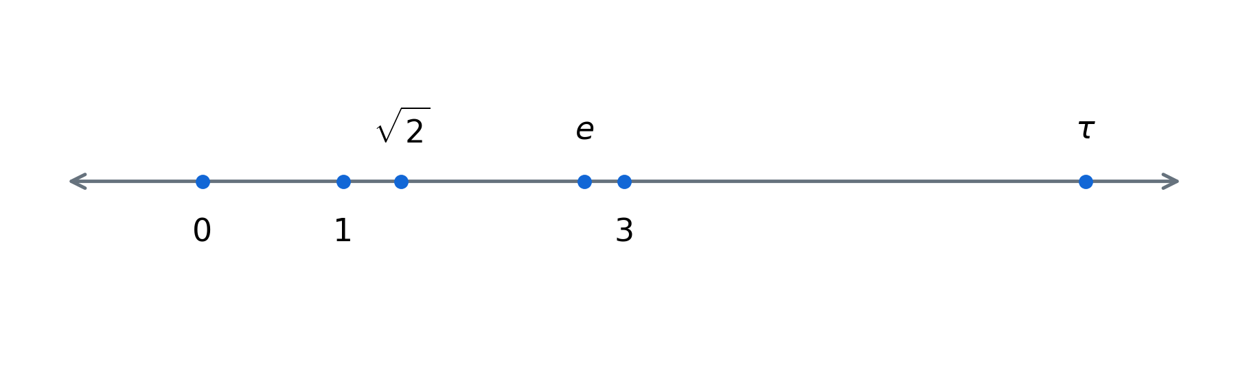
However, in the real numbers, all squares are nonnegative, as mentioned in chapter 1. The square roots of negative numbers are not well-defined with real numbers. So, what does a negative square root mean?
To explore this, Bombelli developed rules for calculating with what we now call imaginary numbers.2 Today we write the imaginary unit as \(i\), and it has the property that
\[\boxed{i^{2} = - 1}\]
So then \(i = \sqrt{- 1}\).
\(i\) does not exist on the real number line, as no number on the real line can square to \(- 1\). \(i\) can be multiplied by a real number, to create any multiple of \(i\), known as imaginary numbers. These multiples work exactly as you would expect, \((2i)^{2} = - 4\), for example. These numbers exist on their own number line, independent of the real numbers. However, the visualization of imaginary numbers as two separate number lines is not the complete story.
At first, the imaginary unit seems like hocus pocus, a quick fix for a problem we can’t solve. In fact, many mathematicians distrusted the concept, and decades later, Descartes used the name “imaginary” for roots that were not “real”.3
However, mathematicians soon discovered that these “imaginary numbers” can actually describe math better than real numbers can. They have deep connections to polynomials, trigonometry, hyperbolic trigonometry, the constant e, and many other wonders of mathematics. So, these “imaginary numbers” have turned out to provide very “real” results.
Complex Numbers
Bombelli went further by developing rules for calculating with these quantities. Today, we describe a complex number as the sum of a real number and an imaginary number, of the general form \(\boxed{a + bi}\), where \(a\) and \(b\) are real numbers. Examples of complex numbers include \(1 + 2i\), \(3 - 4i\) or \(e + \pi i\). Notice that the set of complex numbers includes all real numbers, \(a + 0i\), and all purely imaginary numbers \(0 + bi\).
To visualize this new set of numbers, we need to extend our concept of a number line into two dimensions. We don’t need a number line, we need a number plane. We set up a plane like with regular coordinates, with real numbers on our x-axis, and imaginary numbers on our y-axis.
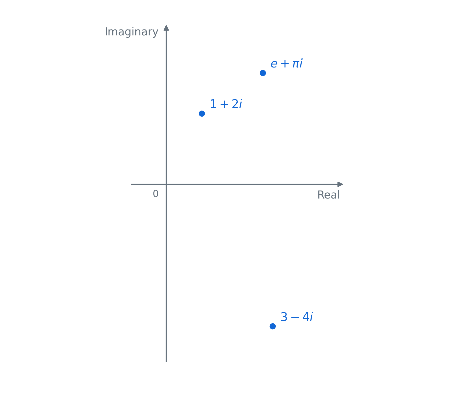
Now, we can represent any complex number as a single point on this plane. Notice how this isn’t a usual x/y plane with an input and output; it is a visual for all complex numbers.
To better describe these numbers, there is some basic terminology I will be using throughout the rest of the book.
Real numbers refer to all numbers without an imaginary component.
Purely imaginary (or just imaginary) numbers are numbers that lie on the imaginary axis (like 2i or \(- 5i\)).
Both imaginary and real numbers are subsets of complex numbers, of the general form \(a + bi\).
The real part of a complex number, notated as \(Re(z)\), is the real number component of the complex number. For example: \(Re(2 + 3i) = 2\)
The imaginary part of a complex number, written as \(Im(z)\), gives the real number that is multiplied by i in the number; for example \(Im( - 5 + 4i) = 4\)
Complex Number Arithmetic
A natural question is: Do our new complex numbers work the same way real numbers do? Will arithmetic work with complex numbers? Do the same laws apply? Fortunately, the answer is yes! However, these operations are visualized much better geometrically, in terms of the complex plane, than algebraically with symbols.
Addition and Subtraction
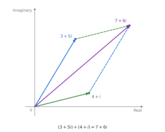
If we want to add two complex numbers, say \((3 + 5i) + (4 + i)\), we can simply combine like terms to get our result \((3 + 4) + (5 + 1)i = 7 + 6i\). A visual way to add two complex numbers is to plot them both in the complex plane:
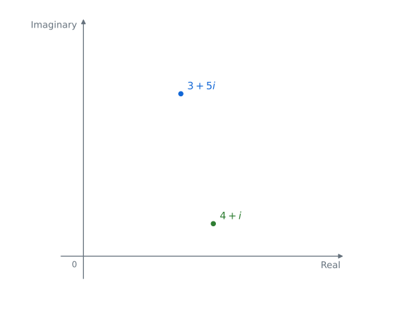
Draw line segments between both points and \((0,0)\).
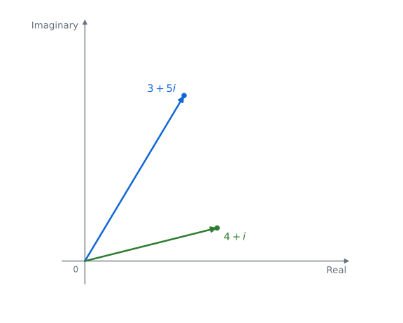
These three points and the answer to our problem will always form a parallelogram, possibly a degenerate one!
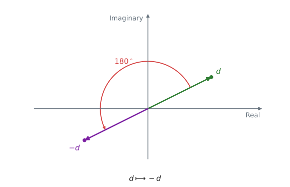
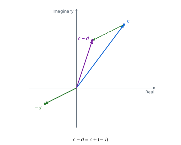
Subtraction works the same way in algebraic terms, and can also be incorporated into our visual. Subtraction of two complex numbers \(c\) and \(d\) is really just adding the opposite, because \(c - d = c + ( - d)\). The negative of a complex number is just the point rotated 180° around the origin.
So, all we need to do to subtract two numbers is just add the negative of the second, as shown:
Multiplication Algebraically
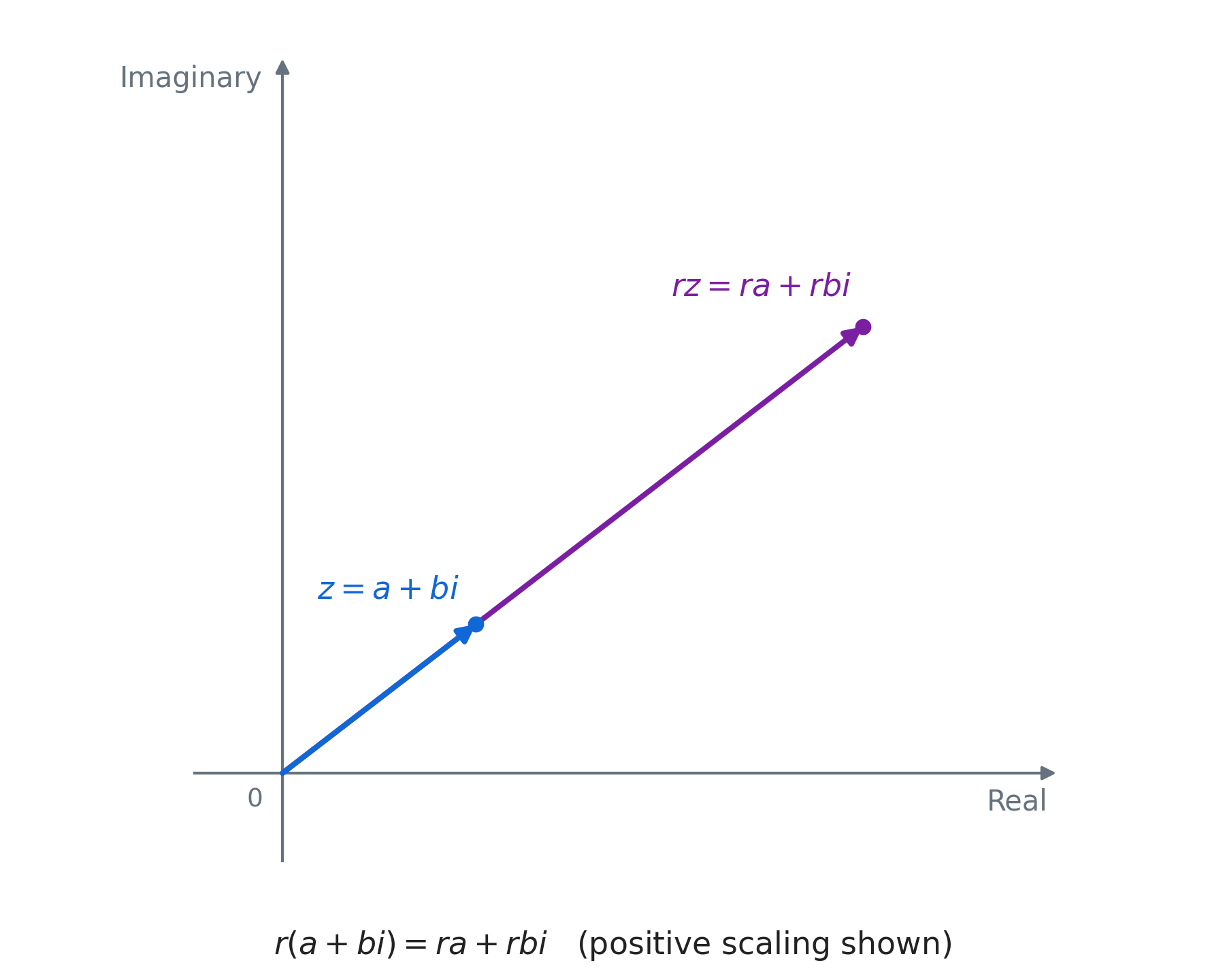
Multiplication of complex numbers is more complicated. Multiplication by a real number is easy, because this is equivalent to scaling the line segment to the origin by the absolute value of the multiplier. A negative multiplier also turns it halfway around the origin, and a zero multiplier sends it to the origin. This is easy because on the real or imaginary axis, if we want to multiply by 3, or 4, or 2.5, we just take the original segment, copy it 3, 4 or 2.5 times, and calculate the distance from there.
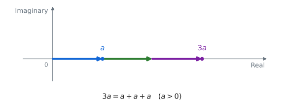
It turns out that this works for all complex numbers. We can see this algebraically by the distributive law:
\(r(a + bi) = ra + rbi\), assuming r is a real number.
What happens if we multiply by an imaginary number? If we multiply a positive real number by \(i\), we end up on the positive imaginary axis. If we multiply a positive imaginary number by \(i\), because \(i^{2} = - 1\), we will end up on the negative real axis.
This pattern continues when we keep multiplying by \(i\); our point “cycles” counterclockwise through all four axis directions.
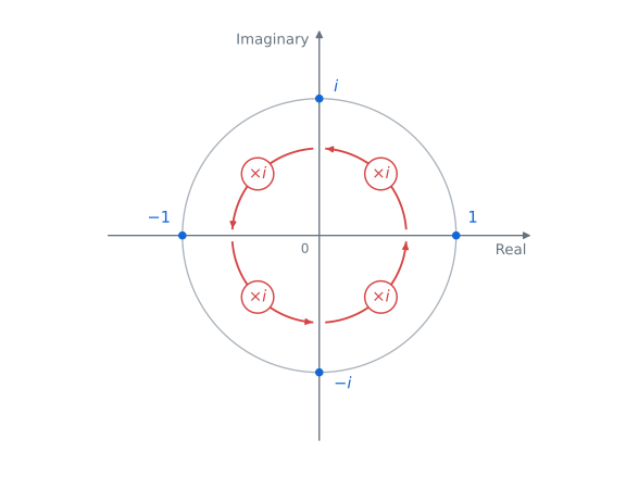
In this light, multiplication by \(i\) can be visualized by a 90° rotation about the origin. However, we have only checked this fact for real and purely imaginary numbers. It just so happens that this applies to all complex numbers. To see why, let’s examine the algebra behind this. Rotation in the Cartesian plane by 90° counterclockwise is equivalent to mapping the point \((x,y)\) to the new point \(( - y,x)\). We can also see this in action for any point, say \((3,4)\):
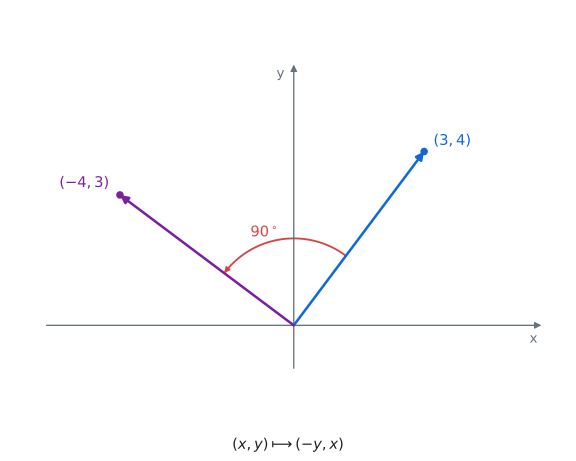
In the complex plane, the x and y coordinates of a point are the real and imaginary parts of a complex number. Multiplying the complex number \((a + bi)\) by \(i\) gives
\[\boxed{i\ (a + bi) = ia + i(ib) = - b + ai}\]
The original real part (our x-coordinate) was a, and our original imaginary part (our y-coordinate) was b. Now our new real part is -b, and our new imaginary part is a, which means this is equivalent to our rotation formula!
This is the same counterclockwise quarter-turn shown in Figure 7.11, so the algebra and the picture describe the same operation.
So, multiplying by a purely imaginary number can be thought of as rotating and scaling any point in the complex plane!
Unfortunately, Bombelli did not know of these magical visuals. Later, Euler developed the algebra, while Caspar Wessel, Argand and Carl Gauss helped establish the geometric picture.4
To multiply two complex numbers, we apply the distributive law and expand, like this:
\[(4 + i)(2 + 3i) = 8 + 2i + 12i + 3i^{2} = 8 - 3 + 14i = 5 + 14i\]
To fully understand multiplication of complex numbers geometrically, we must visualize the complex plane with a new coordinate system.
Up to this point, we have been looking at a point in the plane as being described by two signed coordinates, \(x\) horizontally and \(y\) vertically from the origin (with positive \(y\) pointing upward). This is known as the Cartesian coordinate system, and is very useful for visualizing numbers in the complex plane. However, the polar coordinate system is good at expressing points based on direct distances from the origin, and is perfect for describing complex number multiplication.
The Polar Coordinate System
In polar coordinates, a point is described by a direct distance from the origin, called \(r\), and the angle it makes with the x-axis, called \(\theta\). Both of these numbers provide a complete description of a point, \((r,\theta)\).
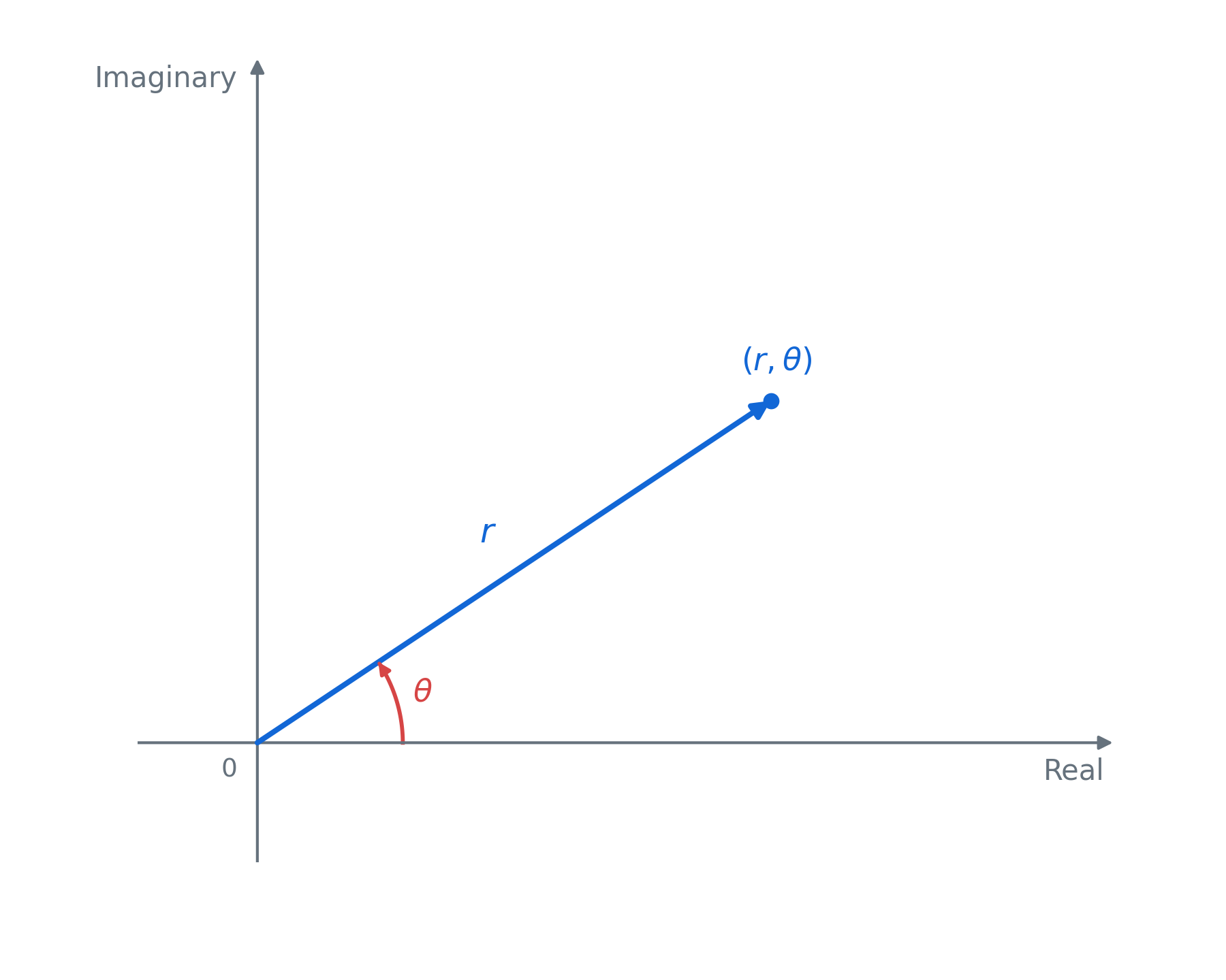
In the context of complex numbers, \(r\) is often called the “magnitude” of a number. It can also be thought of as the absolute value of the number. For real numbers, absolute value is extremely simple: it is just distance from zero in either direction, and is always nonnegative. However, with complex numbers, distance from zero still applies, but it is more complicated to find.
To find \(r\) and θ from the real and imaginary parts of a complex number, we must use trigonometry. To find \(r\), we form a triangle with the origin, where the two legs have lengths \(|x|\) and \(|y|\) (with a degenerate triangle when either is zero), and the hypotenuse has distance \(r\):
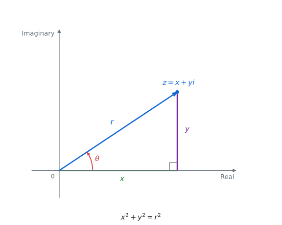
Since this is a right triangle, by the Pythagorean Theorem, \(x^{2} + y^{2} = r^{2}\), so
\[\boxed{r = \sqrt{x^{2} + y^{2}}}\]
For \(x \neq 0\), we can now say that
\[\tan(\theta) = \frac{y}{x}\]
When \(x > 0\) and we choose \(- \pi/2 < \theta < \pi/2\), taking the arctangent gives
\[\arctan\left( \frac{y}{x} \right) = \theta\]
So, for \(x > 0\), the polar coordinates are
\[\left( \sqrt{x^{2} + y^{2}}\ ,\arctan\left( \frac{y}{x} \right) \right)\]
There is one small caveat with this conversion, as negative signs get in the way. For example, if we take the complex number \(3 + 2i\) and its negative \(- 3 - 2i\), applying the conversion suggests they both have the same value of θ, which is \(\theta \approx 0.588\), measured in radians.
In reality, they are 180° apart from each other. The ratio alone loses this quadrant information.
To choose an angle in \(( - \pi,\pi\rbrack\), add \(\pi\) to \(\arctan(y/x)\) when \(x < 0\) and \(y \geq 0\), and subtract \(\pi\) when \(x < 0\) and \(y < 0\). When \(x = 0\), use \(\pi/2\) for \(y > 0\) and \(- \pi/2\) for \(y < 0\). The origin has magnitude zero and no defined angle. Angles that differ by a full turn, \(\tau = 2\pi\) radians, represent the same direction.
Converting back to Cartesian coordinates is simpler, as we can use the sine and cosine functions of theta to get our x and y coordinates. However, these coordinates assume the radius is 1, so we must scale the unit circle up by a factor of \(r\) to get the conversion.
Therefore, the real and imaginary components are \(Re(z) = r\cos(\theta),\ Im(z) = r\sin(\theta)\), where z is a complex number; therefore
\[\boxed{z = r(\cos(\theta) + i\ \sin(\theta))}\]
We can also extend the potential values of the polar radius \(r\) to the negatives (its magnitude is then \(|r|\)), by considering what happens as we decrease \(r\). As we decrease \(r\), the point moves closer and closer to the origin, so if we decrease \(r\) to below 0, it makes sense for the point to continue moving in the same direction. Therefore, this is equivalent to having positive distance, and adding or subtracting 180 degrees from the angle \(( - r,\theta)\) is equivalent to \((r,\theta + 180^{{^\circ}})\).
Therefore, points in polar coordinates can be represented by different ordered pairs. One last thing to keep in mind is that adding 360 degrees (or \(\tau\) radians) doesn’t change the point’s location, so the point \((r,\theta)\) is the same as \((r,\theta + 360^{{^\circ}})\).
Multiplication in Polar Form
Take two nonzero complex numbers, \(z_{1}\) and \(z_{2}\), with magnitudes \(r_{1}\) and \(r_{2}\), and angles \(\theta_{1}\) and \(\theta_{2}\). Multiplying their polar expressions together, we find:
\(z_{1}\ z_{2} = r_{1}r_{2}\lbrack\left( \cos\left( \theta_{1} \right) + i\sin\left( \theta_{1} \right) \right)\ (\cos\left( \theta_{2} \right) + i\sin\left( \theta_{2} \right))\rbrack\)
We can expand out:
\[\left( \cos\left( \theta_{1} \right) + i\sin\left( \theta_{1} \right) \right)\left( \cos\left( \theta_{2} \right) + i\sin\left( \theta_{2} \right) \right)\]
to
\[\cos\left( \theta_{1} \right)\cos\left( \theta_{2} \right) + i\sin\left( \theta_{1} \right)\cos\left( \theta_{2} \right) + i\sin\left( \theta_{2} \right)\cos\left( \theta_{1} \right) + i^{2}\sin\left( \theta_{1} \right)\sin\left( \theta_{2} \right)\]
Collecting like terms, we find
\[\cos\left( \theta_{1} \right)\cos\left( \theta_{2} \right) - \sin\left( \theta_{1} \right)\sin\left( \theta_{2} \right) + i\left( \sin\left( \theta_{1} \right)\cos\left( \theta_{2} \right) + sin\left( \theta_{2} \right)\cos\left( \theta_{1} \right) \right)\]
The forms of the real and imaginary parts are the exact result of the trigonometric angle addition identities in chapter 4.
Recall that
\[\cos(a + b) = \cos(a)\cos(b) - \sin(a)\sin(b)\]
and that
\[\sin(a + b) = \sin(a)\cos(b) + \cos(a)\sin(b)\]
Now, we can use these identities in reverse and express these as a cosine or sine of a sum of angles:
\[\cos\left( \theta_{1} + \theta_{2} \right) + i\sin(\theta_{1} + \theta_{2})\]
Substituting this result into our original multiplication, we find that the result is
\[\boxed{z_{1}\ z_{2} = r_{1\ }r_{2}\lbrack\cos\left( \theta_{1} + \theta_{2} \right) + i\sin(\theta_{1} + \theta_{2})\rbrack}\]
If we call the result \(z_{3}\), the magnitude is \(r_{3} = r_{1}*r_{2}\) and the angle is \({\theta_{3} = \theta}_{1} + \theta_{2}\).
So, to multiply two complex numbers really means multiplying their magnitudes and adding their angles, modulo a full turn! If either factor is zero, the product is zero and has no defined angle.
For example, let’s take two complex numbers, \(3 + 2i\) and \(5 + 4i\), and multiply them together. Algebraically, we find \((3 + 2i)(5 + 4i) = 15 + 10i + 12i + 8\left( i^{2} \right) = 7 + 22i\). To use our visual method, we must convert to polar form.
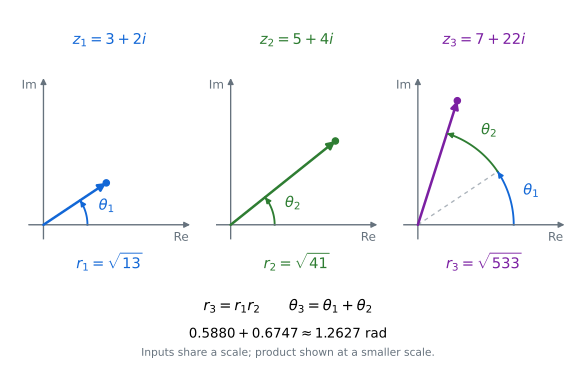
For distances, we find:
\[r_{1} = \sqrt{3^{2} + 2^{2}} = \sqrt{13}\]
while
\[r_{2} = \sqrt{5^{2} + 4^{2}} = \sqrt{41}\]
For our angles, we use arctangent (in radians):
\[\theta_{1} = arctan\left( \frac{2}{3} \right) \approx 0.588\]
and
\[\theta_{2} = arctan\left( \frac{4}{5} \right) \approx 0.6747\]
Multiplying their lengths, we find:
\[r_{3} = \sqrt{13}*\sqrt{41} = \sqrt{533} \approx 23.0868\]
Adding their angles, we find:
\[\theta_{3} \approx 1.2627\ rad\]
The final step is to convert our result back into Cartesian coordinates:
\[a \approx 23.0868*\cos(1.2627) \approx 7\]
and
\[b \approx 23.0868*\sin(1.2627) \approx 22\]
Therefore, our answer is \(7 + 22i\), the same result we got before!
Solutions of Equations
Solving Quadratics
It’s time to see what these complex numbers can do. First and perhaps most important, they can solve many equations that real numbers could not.
Let’s revisit the problematic quadratic equation from chapter 1, \(x^{2} + 5x + 8 = 0\).
We first move the constant, so
\[x^{2} + 5x = - 8\]
Then we add \(\left( \frac{b}{2} \right)^{2}\), which is \(\frac{25}{4}\), to both sides, leaving
\[x^{2} + 5x + \frac{25}{4} = - \frac{7}{4}\]
Completing the square, we find
\[\left( x + \frac{5}{2} \right)^{2} = \frac{- 7}{4}\]
We stopped here because we didn’t know how to take the square root of a negative number, but now that we have imaginary numbers, we can keep on solving!
\[x + \frac{5}{2} = \pm \frac{\sqrt{- 7}}{2} = \pm \frac{\sqrt{7}i}{2}\]
Our solutions are
\(\boxed{x = \frac{- 5 \pm \sqrt{7}i}{2}}\), which we can plot on the complex plane.
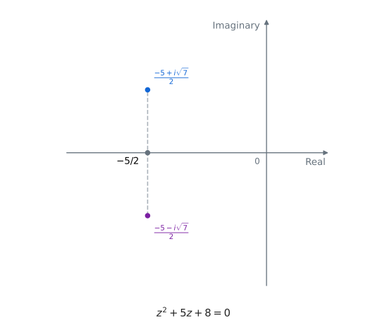
One thing that is interesting about these roots is that they have the same real part, but opposite imaginary parts. Numbers of this form are known as complex conjugates: for any complex number \(a + bi\), \(a - bi\) is its conjugate.
It turns out that this is not a coincidence, and there is a theorem called the Complex Conjugate Theorem that states that for any polynomial with real coefficients and a non-real solution, its conjugate must also be a solution. This can significantly reduce the work in solving polynomials, because once you know one non-real root of such a polynomial, you can instantly find its conjugate.
Solving Cubic Equations
Now that we know how to solve any quadratic equation, let’s shift our attention to cubic equations. The problem we ran into with the casus irreducibilis came up when we tried to solve the resulting quadratic and got stuck. Now, this roadblock is removed with our knowledge of complex numbers. However, before we plug and chug into this formula, we will need some intuition of how square roots and cube roots work in this number system.
Square and Cube Roots
In the real number system, we know that there are two square roots of any positive real number. In the complex number system, every negative real number also has two square roots, so \(\sqrt{- 1} = i\) is the principal square root, while the two solutions of \(D^{2} = - 1\) are \(\pm i\).
Now what does it mean to take the square root of a complex number? Say \(\sqrt{C} = D\), where \(C \neq 0\) and \(D\) is its principal square root. Choose the angle of \(C\) in \(( - \pi,\pi\rbrack\) and the angle of \(D\) in \(( - \pi/2,\pi/2\rbrack\). Then we know that \(D^{2} = C\).
Now we can use our knowledge of complex multiplication to find the magnitudes and angles of these numbers. Therefore,
\[r_{D}\ r_{D} = r_{C}\qquad \left( r_{D} \right)^{2} = r_{C}\]
and
\[\theta_{D} + \theta_{D} = \theta_{C}\qquad {2\theta}_{D} = \theta_{C}\]
Now we can express our unknown polar form of D in terms of C.
\[\sqrt{r_{C}} = r_{D}\qquad \frac{\theta_{C}}{2} = \theta_{D}\]
To take the square root of a complex number, we halve its angle and square root its magnitude. For \(C \neq 0\), the two solutions of \(D^{2} = C\) are \(D\) and \(- D\). When \(C = 0\), there is only one distinct solution, zero, with multiplicity two.
In the real numbers, there is only one cube root of a number. However, using complex numbers, every nonzero number has three different cube roots, in the same sense that it has two square roots. Zero has one distinct cube root, zero, with multiplicity three.
For example, let’s find the three cube roots of 1. This is equivalent to solving the equation
\[x^{3} = 1\qquad x^{3} - 1 = 0\]
We already know \(x = 1\) is a solution, so we can factor \((x - 1)\) out, leaving
\[(x - 1)(x^{2} + x + 1) = 0\]
We can solve the quadratic by completing the square.
Moving the constant:
\[x^{2} + x = - 1\]
Adding \(\frac{1}{4}\) to both sides
\[x^{2} + x + \frac{1}{4} = - \frac{3}{4}\]
Collapsing into one square term
\[\left( x + \frac{1}{2} \right)^{2} = - \frac{3}{4}\]
Taking square roots of both sides
\[x + \frac{1}{2} = \pm \frac{\sqrt{3}}{2}i\]
Moving the constant leaves two solutions
\[\boxed{x = - \frac{1}{2} \pm \frac{\sqrt{3}}{2}i}\]
We can plot our three cube roots in the complex plane, which looks like this:
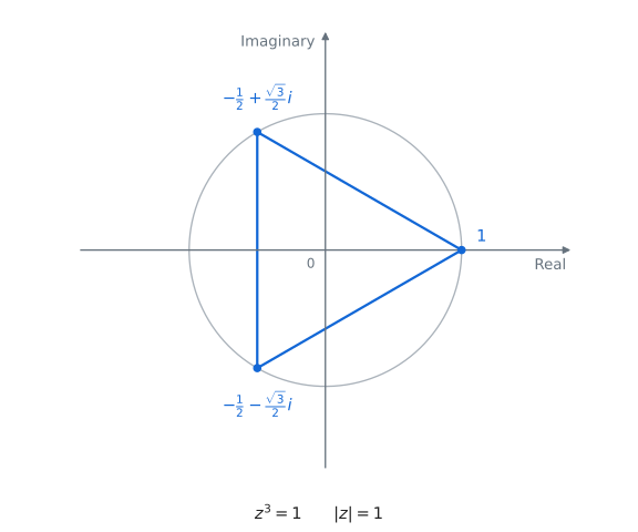
These numbers are known as the cube roots of unity (unity meaning one).
One important point is that the two complex roots are conjugates. To find the cube roots of any real number, we simply extract the real cube root, and multiply by the other roots of unity.
For \(C \neq 0\), we apply the same logic as square roots and choose one cube root \(D\) with \(D^{3} = C\) by taking
\[\boxed{r_{D} = \sqrt[3]{r_{C}}}\qquad \boxed{\theta_{D} = \frac{1}{3}\theta_{C}}\]
This gives us one of the cube roots, and to find the others, we multiply by the cube roots of unity, just like real numbers. So, because the roots of unity have a magnitude of 1, you are rotating the number by \(\frac{1}{3}\) and \(\frac{2}{3}\) of a full circle, or by \(\frac{\tau}{3}\) and \(\frac{2\tau}{3}\) radians.
A Cubic With Three Real Roots
With our knowledge of complex roots, we are now ready to tackle the casus irreducibilis, just as Bombelli did in his Algebra, published in 1572.5 Let’s try and solve a cubic with three real roots, \(x^{3} - 14x - 8 = 0\). We can easily check by guessing that one of the solutions is 4. Plugging into the depressed cubic formula, we find
\[x = \sqrt[3]{4 + \sqrt{16 - \frac{2744}{27}}} + \sqrt[3]{4 - \sqrt{16 - \frac{2744}{27}}}\]
These square roots of negative numbers made Cardano’s cubic formula seem unusable for some cubics. However, we can just keep solving!
Simplifying the square roots:
\[x = \sqrt[3]{4 + \frac{34\sqrt{6}}{9}i} + \sqrt[3]{4 - \frac{34\sqrt{6}}{9}i}\]
Now we can convert to polar form and calculate the cube roots.
The magnitude of both numbers (complex conjugates have the same magnitude) is:
\[\sqrt{4^{2} + \left( \frac{34\sqrt{6}}{9} \right)^{2}} = \sqrt{\frac{2744}{27}} \approx 10.0812\]
Now we can also calculate the angle of the first:
\[\arctan\left( \frac{34\sqrt{6}}{9} \div 4 \right) = \arctan\left( \frac{34\sqrt{6}}{36} \right) \approx 1.1628\ rad\]
The angle of the second is simply the negative of the first because they are complex conjugates. Extracting cube roots, we find that \(r_{1} = r_{2} \approx 2.1603\), and \(\theta_{1} \approx 0.3876\),
\(\theta_{2} \approx - 0.3876\). These cube roots are conjugates as well!
Converting back to Cartesian form gives
\[x = 2 + \frac{\sqrt{6}}{3}i + 2 - \frac{\sqrt{6}}{3}i = 4\]
We derive the solution \(x = 4\), which checks out in the original equation.
To find the other two solutions to this equation, we factor out \((x - 4)\) from the cubic equation.
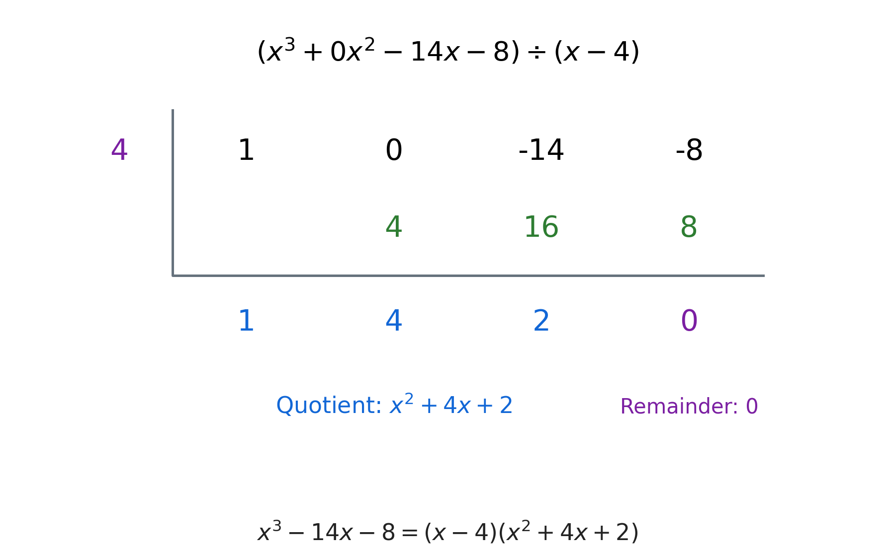
\[x^{2} + 4x + 2 = 0\]
We can solve this by the quadratic formula:
\[x_{2,3} = \frac{- 4 \pm \sqrt{4^{2} - 4(2)}}{2}\]
\[x_{2,3} = - 2 \pm \sqrt{2}\]
Approximate values are:
\[x_{2} \approx - 0.5858\]
\[x_{3} \approx - 3.4142\]
The General Cubic
What about the other solutions in the general case?
Looking at the cubic formula, each nonzero radicand has three complex cube roots, so it looks like there are actually nine possible formulas! But there are three roots of the cubic equation, counting multiplicity. To see why only three of the formulas work out, we need to look back at how we derived the formula. All of the algebraic manipulations in real numbers also work in complex numbers (but the geometry of the cubes doesn’t extend well to negative or complex numbers). In Cardano’s derivation (but this also applies to my method), we need to extract the cube root of the expression \(\frac{q}{2} + \sqrt{\left( \frac{q}{2} \right)^{2} + \left( \frac{p}{3} \right)^{3}}\) to isolate y. (The minus solution also works).6
So, we obtain
\[y = \sqrt[3]{\frac{q}{2} + \sqrt{\left( \frac{q}{2} \right)^{2} + \left( \frac{p}{3} \right)^{3}}}\]
For a nonzero radicand, there are actually three choices for \(y\). Whenever both radicals are real and compatible, we recover the real-valued calculation from chapter 2, but what if we use the other complex choices?
Choose the square-root sign so that \(y\) is nonzero, and call this chosen cube root \(y_{0}\). Read this cube-root radical below as \(y_{0}\). The case \(p = q = 0\) will be handled separately.
Setting
\[y = \left( - \frac{1}{2} + \frac{\sqrt{3}}{2}i \right)\sqrt[3]{\frac{q}{2} + \sqrt{\left( \frac{q}{2} \right)^{2} + \left( \frac{p}{3} \right)^{3}}}\]
we can obtain our second solution. Looking back at our system, when plugging in \(y^{3}\), we find the exact same equation for \(z^{3}\), except we also have three different solution possibilities for z.
\[z^{3} + q = \frac{q}{2} + \sqrt{\left( \frac{q}{2} \right)^{2} + \left( \frac{p}{3} \right)^{3}}\]
\[z^{3} = - \frac{q}{2} + \sqrt{\left( \frac{q}{2} \right)^{2} + \left( \frac{p}{3} \right)^{3}}\]
Now, when we extract the cube root, there are also three possibilities!
We must remember that the first equation in the system, \(p = 3yz\), must also be satisfied. It is not enough for \(3yz\) to be real: it must equal \(p\). Starting with the chosen \(y_{0} \neq 0\), take \(z_{0} = p/\left( 3y_{0} \right)\), and read the second cube-root radical as this compatible \(z_{0}\). Then \(y_{0}z_{0} = p/3\). If \(y_{0}\) is multiplied by one nontrivial cube root of unity, \(z_{0}\) must be multiplied by its inverse. Therefore:
\[z = \left( - \frac{1}{2} - \frac{\sqrt{3}}{2}i \right)\sqrt[3]{- \frac{q}{2} + \sqrt{\left( \frac{q}{2} \right)^{2} + \left( \frac{p}{3} \right)^{3}}}\]
The same logic holds true if we assumed y had the third possible cube root. Starting from this compatible pair, multiply its two members by inverse roots of unity. These pairings preserve \(yz = p/3\), including when the starting pair is non-real; the cube-root branches cannot be selected independently.
So, our three solutions, counting multiplicity, for the equation
\[ax^{3} + bx^{2} + cx + d = 0\]
Can be found by setting
\[p = c/a - b^{2}/\left( 3a^{2} \right)\qquad q = 2b^{3}/\left( 27a^{3} \right) - bc/\left( 3a^{2} \right) + d/a\]
and
\[\boxed{D = (q/2)^{2} + (p/3)^{3}}\]
In all six displayed versions, call the first cube-root term \(U\) and the second \(V\).
Choose a square root of \(D\) and a nonzero cube root \(U\) of \(- q/2 + \sqrt{D}\), then take \(V = - p/(3U)\).
If the first radicand is zero, reverse the square-root sign.
This makes \(V\) a cube root of \(- q/2 - \sqrt{D}\) and enforces \(UV = - p/3\).
The three solutions are
\[U + V - b/(3a)\qquad \ \ \ \ \ \ \omega U + \omega^{2}V - b/(3a)\qquad \omega^{2}U + \omega V - b/(3a)\]
where \(\omega = - 1/2 + \left( \sqrt{3}/2 \right)i\)
If \(p = q = 0\), all three roots coincide at \(- b/(3a)\). When \(p = 0\) but \(q \neq 0\), one of \(U,V\) is zero; the same three expressions still give the complete root family:
\[x_{1} = \sqrt[3]{- \frac{b^{3}}{27a^{3}} + \frac{bc}{6a^{2}} - \frac{d}{2a} + \sqrt{\left( \frac{b^{3}}{27a^{3}} - \frac{bc}{6a^{2}} + \frac{d}{2a} \right)^{2} + \left( - \frac{b^{2}}{9a^{2}} + \frac{c}{3a} \right)^{3}}}\]
\[+ \sqrt[3]{- \frac{b^{3}}{27a^{3}} + \frac{bc}{6a^{2}} - \frac{d}{2a} - \sqrt{\left( \frac{b^{3}}{27a^{3}} - \frac{bc}{6a^{2}} + \frac{d}{2a} \right)^{2} + \left( - \frac{b^{2}}{9a^{2}} + \frac{c}{3a} \right)^{3}}} - \frac{b}{3a}\]
\[x_{2} = \left( - \frac{1}{2} + \frac{\sqrt{3}}{2}i \right)\sqrt[3]{- \frac{b^{3}}{27a^{3}} + \frac{bc}{6a^{2}} - \frac{d}{2a} + \sqrt{\left( \frac{b^{3}}{27a^{3}} - \frac{bc}{6a^{2}} + \frac{d}{2a} \right)^{2} + \left( - \frac{b^{2}}{9a^{2}} + \frac{c}{3a} \right)^{3}}}\]
\[+ \left( - \frac{1}{2} - \frac{\sqrt{3}}{2}i \right)\sqrt[3]{- \frac{b^{3}}{27a^{3}} + \frac{bc}{6a^{2}} - \frac{d}{2a} - \sqrt{\left( \frac{b^{3}}{27a^{3}} - \frac{bc}{6a^{2}} + \frac{d}{2a} \right)^{2} + \left( - \frac{b^{2}}{9a^{2}} + \frac{c}{3a} \right)^{3}}} - \frac{b}{3a}\]
\[x_{3} = \left( - \frac{1}{2} - \frac{\sqrt{3}}{2}i \right)\sqrt[3]{- \frac{b^{3}}{27a^{3}} + \frac{bc}{6a^{2}} - \frac{d}{2a} + \sqrt{\left( \frac{b^{3}}{27a^{3}} - \frac{bc}{6a^{2}} + \frac{d}{2a} \right)^{2} + \left( - \frac{b^{2}}{9a^{2}} + \frac{c}{3a} \right)^{3}}}\]
\[+ \left( - \frac{1}{2} + \frac{\sqrt{3}}{2}i \right)\sqrt[3]{- \frac{b^{3}}{27a^{3}} + \frac{bc}{6a^{2}} - \frac{d}{2a} - \sqrt{\left( \frac{b^{3}}{27a^{3}} - \frac{bc}{6a^{2}} + \frac{d}{2a} \right)^{2} + \left( - \frac{b^{2}}{9a^{2}} + \frac{c}{3a} \right)^{3}}} - \frac{b}{3a}\]
Another method to solve the example equation is plugging into the above formulas:
\[x_{2} = \left( - \frac{1}{2} + \frac{\sqrt{3}}{2}i \right)\left( 2 + \frac{\sqrt{6}}{3}i \right) + \left( - \frac{1}{2} - \frac{\sqrt{3}}{2}i \right)(2 - \frac{\sqrt{6}}{3}i)\]
\[x_{3} = \left( - \frac{1}{2} - \frac{\sqrt{3}}{2}i \right)\left( 2 + \frac{\sqrt{6}}{3}i \right) + \left( - \frac{1}{2} + \frac{\sqrt{3}}{2}i \right)(2 - \frac{\sqrt{6}}{3}i)\]
After distributing and collecting like terms, all of the imaginary terms cancel out, and we find:
\[x_{2} = - 2 - \sqrt{3}(\frac{\sqrt{6}}{3})\]
\[x_{3} = - 2 + \sqrt{3}(\frac{\sqrt{6}}{3})\]
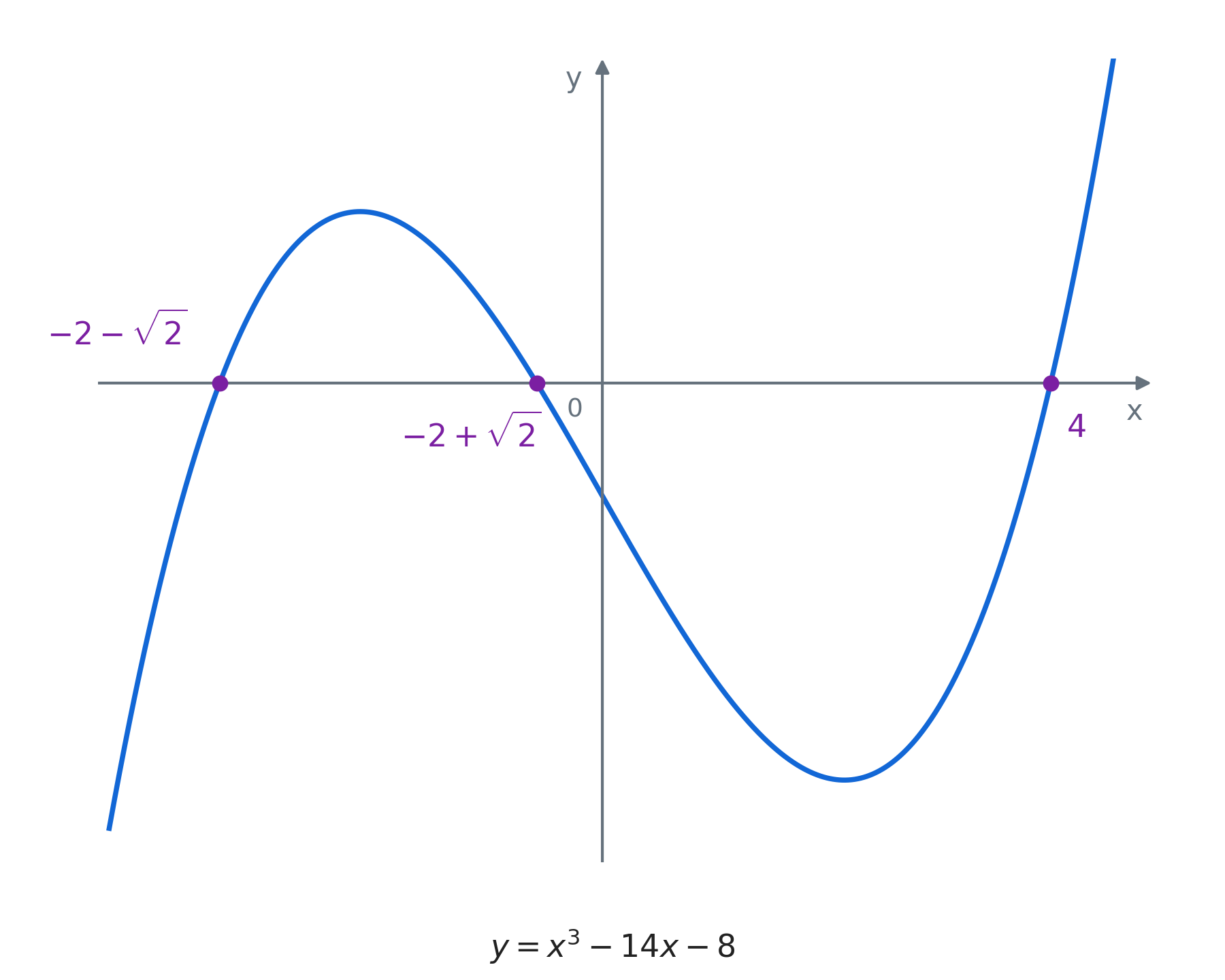
Therefore, all three real solutions to the cubic \(x^{3} - 14x - 8 = 0\) are
\[x_{1} = 4\]
\[x_{2} \approx - 3.4142\]
\[x_{3} \approx - 0.5858\]
We can clearly see these solutions on the graph of the cubic equation:
A Cubic With One Real Root and Two Complex Roots
Now, let’s see how the cubic formula can solve a cubic with one real root and two complex roots. For example, let’s take the cubic
\[x^{3} - 5x^{2} + 2x - 1 = 0\]
Plugging into the original cubic formula to find the real root gives:
\[x_{1} = \sqrt[3]{\frac{187}{54} + \frac{\sqrt{93}}{6}} + \sqrt[3]{\frac{187}{54} - \frac{\sqrt{93}}{6}} + \frac{5}{3}\]
An approximate answer is \(x_{1} \approx 4.6135\)
One approach to finding the other roots would be simply factoring out our known root to get a quadratic, and solving the quadratic to find the other solutions. However, we can instead find the other solutions by multiplying the cube roots by the roots of unity, in the method shown above.
After approximating the cube roots, our second solution should equal
\[x_{2} \approx \left( - \frac{1}{2} + \frac{\sqrt{3}}{2}i \right)(1.718) + \left( - \frac{1}{2} - \frac{\sqrt{3}}{2}i \right)(1.2289) + \frac{5}{3}\]
Distributing and combining like terms, we find:
\[x_{2} \approx 0.1933 + 0.4236i\]
We know that the third solution is simply the complex conjugate of the second; therefore
\[x_{3} \approx 0.1933 - 0.4236i\]
Using the cubic formula would have produced the same result.
So, our complete solution set for the cubic \(x^{3} - 5x^{2} + 2x - 1 = 0\) is:
\[x_{1} \approx 4.6135\]
\[x_{2} \approx 0.1933 + 0.4236i\]
\[x_{3} \approx 0.1933 - 0.4236i\]
The Roots of Unity
The Fourth Roots of Unity
Now that we know how to find the three solutions to any cubic equation (even the casus irreducibilis), let’s explore more about the roots of unity. We know that the cube roots of unity provide the three cube roots of a number, so would higher roots of unity do the same?
For fourth roots, we know that they are simply a composition of two square roots, \(\sqrt[4]{n} = \sqrt{\sqrt{n}}\). For positive real \(n\), the equation \(x^{4} = n\) has two real solutions, obtained by taking both signs of the outer square root. For negative real \(n\) it has no real solutions. However, we are ignoring the possibility of the inner square root being negative, because this does not work in real numbers.
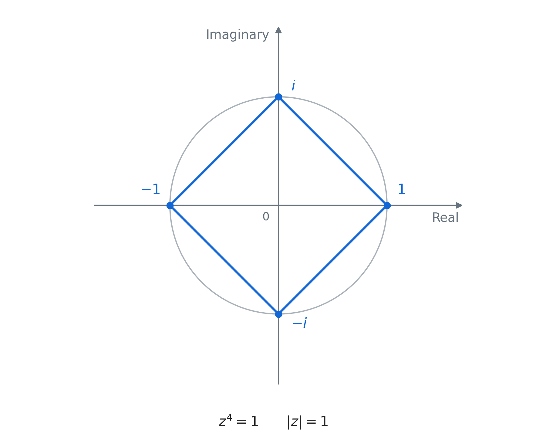
In complex numbers, every nonzero \(n\) has four distinct fourth roots, being \(\sqrt[4]{n}\), \(- \sqrt[4]{n}\), \(i\sqrt[4]{n}\), \(- i\sqrt[4]{n}\). Here the radical denotes its principal value. For \(n = 0\), zero is the only distinct fourth root, with multiplicity four. From this, we derive that the fourth roots of unity are 1, -1, i, and -i. When plotting these in the complex plane, they form a square.
The Fifth Roots of Unity
Because the cube roots of unity formed a triangle in the complex plane, and the fourth roots formed a square, will the fifth roots form a pentagon of some form?
Finding the fifth roots of unity requires solving the equation \(x^{5} = 1\), or \(x^{5} - 1 = 0\). We already know that 1 is a solution, so we can factor out \((x - 1)\), leaving us with
\[\boxed{(x - 1)\left( x^{4} + x^{3} + x^{2} + x + 1 \right) = 0}\]
The quartic on the right will provide the other four roots of unity. We recognize the quartic as a symmetric quartic equation, since all the coefficients are 1.
Since \(x = 0\) is not a root, the first step is to divide by \(x^{2}\), making the equation
\[x^{2} + x + 1 + \frac{1}{x} + \frac{1}{x^{2}} = 0\]
Now, we can substitute \(z = x + \frac{1}{x}\), and \(z^{2} = x^{2} + 2 + \frac{1}{x^{2}}\).
\[z^{2} + z - 1 = 0\]
Solving for z using the quadratic formula, we find two solutions for z:
\[z = \frac{- 1 \pm \sqrt{5}}{2}\]
These are the golden ratio and its algebraic conjugate (which I will write as \(\Phi_{c} = \left( 1 - \sqrt{5} \right)/2 = 1 - \Phi\)), each minus 1:
\[z_{1} = \Phi - 1\]
\[z_{2} = \Phi_{c} - 1\]
We can rewrite \(z_{2}\) using the golden ratio identities in chapter 1:
\[z_{2} = - \Phi\]
Therefore, we have two equations to solve which will provide four overall solutions to the quartic:
\[x + \frac{1}{x} = - \Phi\]
\[x + \frac{1}{x} = \Phi - 1\]
Multiplying by x in equations 1 and 2 yields:
\[x^{2} + 1 = - \Phi x\]
\[x^{2} + 1 = (\Phi - 1)x\]
Moving everything to one side:
\[x^{2} + \Phi x + 1 = 0\]
\[x^{2} + (1 - \Phi)x + 1 = 0\]
Solving each by the quadratic formula gives four solutions for the quartic, and our other four roots of unity:
\[\boxed{x_{1,2} = \frac{- \Phi \pm \sqrt{\Phi^{2} - 4}}{2}}\]
\[\boxed{x_{3,4} = \frac{\Phi - 1 \pm \sqrt{{(1 - \Phi)}^{2} - 4}}{2}}\]
From the original quadratic that defined the golden ratio, we know that \(\Phi^{2} - \Phi - 1 = 0\); therefore \(\Phi^{2} = \Phi + 1\). The same thing is true for the other solution \(1 - \Phi\). Now we can simplify our roots using this equality.
\[x_{1,2} = \frac{- \Phi \pm \sqrt{\Phi - 3}}{2}\]
\[x_{3,4} = \frac{\Phi - 1 \pm \sqrt{- \Phi - 2}}{2}\]
The approximate values of each of the roots are
\[x_{1,2} \approx - 0.809 \pm 0.5878i\]
\[x_{3,4} \approx 0.309 \pm 0.9511i\]
Plotting all five roots in the complex plane forms:
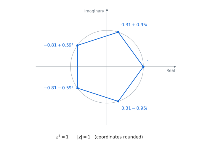
A perfect pentagon!!
In fact, for \(n \geq 3\), the nth roots of unity will form a regular polygon in the complex plane with \(n\) sides. For \(n = 1\) there is one point, 1; for \(n = 2\) there are two antipodal points, 1 and \(- 1\). One final note is that for every positive integer \(n\), all of the nth roots of unity have a magnitude of 1, and their angles are the multiples \(k\frac{\tau}{n}\) for \(k = 0,1,\ldots,n - 1\).
As we have seen, the roots of unity are a fascinating topic in the field of complex numbers, which seem to have a beautiful inherent structure.
What happens if we multiply two of these roots of unity? For the same \(n\), both roots have magnitude 1, so their product still has magnitude 1. Each angle is a whole-number multiple of one full turn divided by \(n\). Multiplying adds these angles, so the new angle is another whole-number multiple of that same step. We can remove any complete turns without changing the number. The product therefore lands on one of the vertices of the same regular polygon: another nth root of unity!
Solving the Quartic With Complex Solutions
Ferrari’s Method
Let’s apply Ferrari’s method from Chapter 3 to
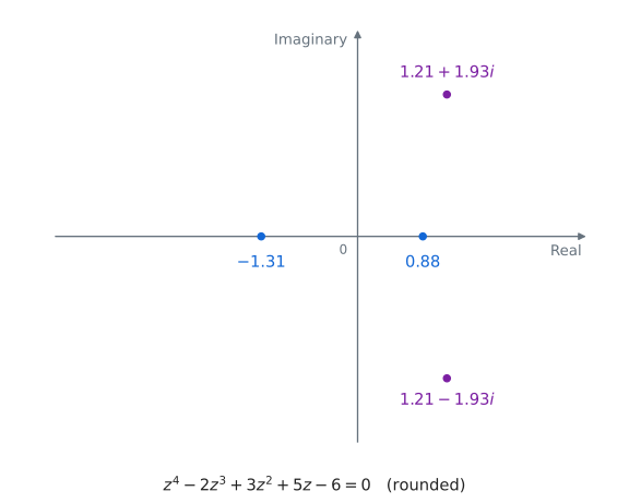
\[x^{4} - 2x^{3} + 3x^{2} + 5x - 6 = 0\]
Substituting \(x = w + \frac{1}{2}\) gives \(w^{4} + \frac{3}{2}w^{2} + 7w - \frac{47}{16} = 0\), so \(p = \frac{3}{2}\), \(q = 7\), and \(r = - \frac{47}{16}\).
For the right side to become a perfect square, z must satisfy
\[64z^{3} + 240z^{2} + 476z - 143 = 0\]
We use its only real root, \(z \approx 0.2630766598\). The cube roots in the exact expression for z below are real cube roots.
Taking square roots as in Ferrari’s method gives
\[w^{2} + \frac{3}{2} + z = \pm \left( \sqrt{\frac{3}{2} + 2z}\, w - \frac{7}{2\sqrt{\frac{3}{2} + 2z}} \right)\]
The minus sign gives a quadratic with two real solutions. The plus sign gives the quadratic
\[w^{2} - \sqrt{\frac{3}{2} + 2z}\, w + \frac{3}{2} + z + \frac{7}{2\sqrt{\frac{3}{2} + 2z}} = 0\]
Completing the square, we obtain the equation
\[\left( w - \sqrt{\ \frac{3}{8} + \frac{1}{2}z} \right)^{2} = - \frac{9}{8} - \frac{1}{2}z - \frac{7}{2\sqrt{\frac{3}{2} + 2z}}\]
The right side is negative, but now we can keep on solving with no problems.
\[w - \sqrt{\ \frac{3}{8} + \frac{1}{2}z} = \pm \sqrt{- \frac{9}{8} - \frac{1}{2}z - \frac{7}{2\sqrt{\frac{3}{2} + 2z}}}\]
Factoring out all the minus signs into \(\sqrt{- 1}\), which is i:
\[w - \sqrt{\ \frac{3}{8} + \frac{1}{2}z} = \pm \sqrt{\frac{9}{8} + \frac{1}{2}z + \frac{7}{2\sqrt{\frac{3}{2} + 2z}}}i\]
\[w = \sqrt{\ \frac{3}{8} + \frac{1}{2}z} \pm \sqrt{\frac{9}{8} + \frac{1}{2}z + \frac{7}{2\sqrt{\frac{3}{2} + 2z}}}i\]
These are the other two “hidden” solutions to our depressed quartic in terms of w. Although the topic of shifting graphs in the complex plane is more advanced than what is covered in this book, the algebraic expression of \(x = w + \frac{1}{2}\) still holds.
Therefore, our other solutions to the equation are:
\[\boxed{x_{3,4} = \frac{1}{2} + \sqrt{\ \frac{3}{8} + \frac{1}{2}z} \pm \sqrt{\frac{9}{8} + \frac{1}{2}z + \frac{7}{2\sqrt{\frac{3}{2} + 2z}}}i}\]
Plugging in for z gives these final expressions:
\[x_{3,4} = \frac{1}{2} + \sqrt{\ \frac{3}{8} + \frac{1}{2}\left( \frac{1}{2\sqrt[3]{6}}\sqrt[3]{183 + 7\sqrt{\frac{2159}{3}}} + \frac{1}{2\sqrt[3]{6}}\sqrt[3]{183 - 7\sqrt{\frac{2159}{3}}} - \frac{5}{4} \right)} \]\(\pm \sqrt{\frac{9}{8} + \frac{1}{2}\left( \frac{1}{2\sqrt[3]{6}}\sqrt[3]{183 + 7\sqrt{\frac{2159}{3}}} + \frac{1}{2\sqrt[3]{6}}\sqrt[3]{183 - 7\sqrt{\frac{2159}{3}}} - \frac{5}{4} \right) + \frac{7}{2\sqrt{\frac{3}{2} + 2\left( \frac{1}{2\sqrt[3]{6}}\sqrt[3]{183 + 7\sqrt{\frac{2159}{3}}} + \frac{1}{2\sqrt[3]{6}}\sqrt[3]{183 - 7\sqrt{\frac{2159}{3}}} - \frac{5}{4} \right)}}}i\)
\[x_{3,4} = \frac{1}{2} + \sqrt{- \frac{1}{4} + \frac{1}{4\sqrt[3]{6}}\sqrt[3]{183 + 7\sqrt{\frac{2159}{3}}} + \frac{1}{4\sqrt[3]{6}}\sqrt[3]{183 - 7\sqrt{\frac{2159}{3}}}} \]\(\pm \sqrt{+ \frac{1}{2} + \frac{1}{4\sqrt[3]{6}}\sqrt[3]{183 + 7\sqrt{\frac{2159}{3}}} + \frac{1}{4\sqrt[3]{6}}\sqrt[3]{183 - 7\sqrt{\frac{2159}{3}}} + \frac{7}{2\sqrt{- 1 + \frac{1}{\sqrt[3]{6}}\sqrt[3]{183 + 7\sqrt{\frac{2159}{3}}} + \frac{1}{\sqrt[3]{6}}\sqrt[3]{183 - 7\sqrt{\frac{2159}{3}}}}}}i\)
Approximations of these complex solutions are:
\(x_{3,4} \approx 1.2117 \pm 1.9275i\)
And here is the graph of all four solutions in the complex plane:
Descartes’ Method
Now let’s apply Descartes’ method from Chapter 3 to
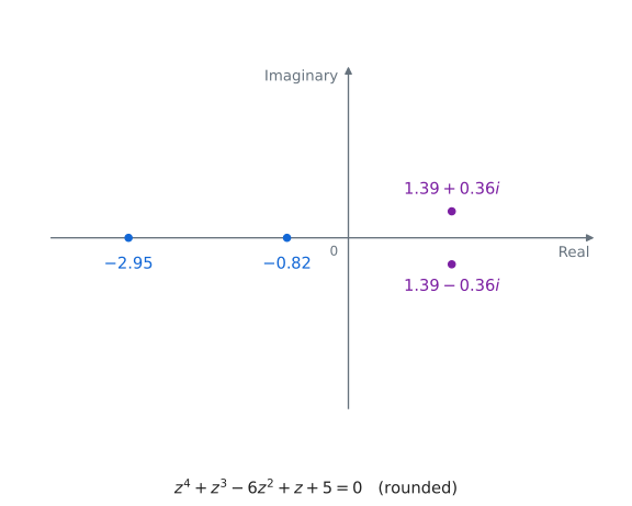
\[x^{4} + x^{3} - 6x^{2} + x + 5 = 0\]
Substituting \(x = w - \frac{1}{4}\) gives \(w^{4} - \frac{51}{8}w^{2} + \frac{33}{8}w + \frac{1117}{256} = 0\).
To factor this as \(\left( w^{2} + kw + l \right)\left( w^{2} - kw + m \right) = 0\), we set \(j = k^{2}\).
The cubic from Descartes’ method becomes \(64j^{3} - 816j^{2} + 1484j - 1089 = 0\).
Its only real root is \(j \approx 10.7382224205\), and we choose \(k = \sqrt{j} > 0\).
Then \(l = \frac{j - 51/8 - 33/(8k)}{2}\) and \(m = \frac{j - 51/8 + 33/(8k)}{2}\)
The cube roots in the exact expressions below are real cube roots.
The quadratic \(w^{2} + kw + l = 0\) gives two real solutions.
The other quadratic is \(w^{2} - kw + m = 0\), and it has the complex solutions of
\[w = \frac{k}{2} \pm \frac{1}{2}\sqrt{k^{2} - 4m}\]
Because the expression \(k^{2} - 4m\) is negative, we can factor out a \(\sqrt{- 1}\) from the radical, and factor in the 1/2, leaving:
\[w = \frac{k}{2} \pm \sqrt{- \frac{k^{2}}{4} + m}i\]
Plugging in for k and m:
\[w = \frac{1}{2}\sqrt{\sqrt[3]{\frac{324 + \sqrt{15603}}{9}} + \sqrt[3]{\frac{324 - \sqrt{15603}}{9}} + \frac{17}{4}} \]\(\pm \sqrt{- \frac{1}{4}\left( \sqrt[3]{\frac{324 + \sqrt{15603}}{9}} + \sqrt[3]{\frac{324 - \sqrt{15603}}{9}} + \frac{17}{4} \right) + \left( \sqrt[3]{\frac{324 + \sqrt{15603}}{72}} + \sqrt[3]{\frac{324 - \sqrt{15603}}{72}} + \frac{33}{16\left( \sqrt{\sqrt[3]{\frac{324 + \sqrt{15603}}{9}} + \sqrt[3]{\frac{324 - \sqrt{15603}}{9}} + \frac{17}{4}} \right)} - \frac{17}{16} \right)}i\)
Simplifying:
\[w_{3,4} = \sqrt{\sqrt[3]{\frac{324 + \sqrt{15603}}{576}} + \sqrt[3]{\frac{324 - \sqrt{15603}}{576}} + \frac{17}{16}} \]\(\pm \frac{1}{2}\sqrt{\sqrt[3]{\frac{324 + \sqrt{15603}}{9}} + \sqrt[3]{\frac{324 - \sqrt{15603}}{9}} + \frac{33}{4\left( \sqrt{\sqrt[3]{\frac{324 + \sqrt{15603}}{9}} + \sqrt[3]{\frac{324 - \sqrt{15603}}{9}} + \frac{17}{4}} \right)} - \frac{17}{2}}i\)
These are the other solutions to our depressed quartic.
Remembering \(x = w - \frac{1}{4}\), we shift back to find our other complex roots:
\[x_{3,4} = - \frac{1}{4} + \sqrt{\sqrt[3]{\frac{324 + \sqrt{15603}}{576}} + \sqrt[3]{\frac{324 - \sqrt{15603}}{576}} + \frac{17}{16}} \]\(\pm \frac{1}{2}\sqrt{\sqrt[3]{\frac{324 + \sqrt{15603}}{9}} + \sqrt[3]{\frac{324 - \sqrt{15603}}{9}} + \frac{33}{4\left( \sqrt{\sqrt[3]{\frac{324 + \sqrt{15603}}{9}} + \sqrt[3]{\frac{324 - \sqrt{15603}}{9}} + \frac{17}{4}} \right)} - \frac{17}{2}}i\)
These complex roots are the “hidden” solutions to the quartic \(x^{4} + x^{3} - 6x^{2} + x + 5 = 0\), and were findable by using the same techniques with knowledge of complex numbers!
The approximate values for these complex roots are
\[\boxed{x_{3,4} \approx 1.3885 \pm 0.3556i}\]
Here are all four solutions plotted in the complex plane:
The Fundamental Theorem of Algebra
We have seen complex numbers come to the rescue again and again. Quadratics, cubics, and quartics that seemed to be missing solutions turned out to have them when we allowed complex numbers. But does that work for every polynomial, or have we just been lucky so far?
The Fundamental Theorem of Algebra says that every nonconstant polynomial of degree \(n\) with complex coefficients has exactly \(n\) complex roots when we count repeated roots according to their multiplicity. For example, \(x^{2} + 1 = 0\) has the two roots \(i\) and \(- i\). The cubic \((x - 2)^{2}(x + 1) = 0\) has roots \(2\), \(2\), and \(- 1\). Two roots happen to have the same value, but we still count three roots altogether.
Something deeper is happening here. A polynomial can have real coefficients and still force its solutions into the complex numbers, as we saw in our earlier equations. But once we allow complex numbers, every nonconstant polynomial has a complex root. We can factor out its linear term and are left with a polynomial of smaller degree. Repeating this process eventually breaks the whole polynomial into linear factors. Mathematicians describe this by saying that the complex numbers are algebraically closed.
There is one important distinction. This theorem tells us that roots exist; it does not promise a simple formula for calculating them. In Chapter 3, we saw that there is no general formula for the quintic using only arithmetic operations and radicals. That doesn’t mean the five complex roots of a quintic are missing. It means there is no formula of that particular kind that produces them for every quintic.
We began this chapter with something that looked like a strange trick for taking the square root of a negative number. Now we can see that the complex numbers are much more than a trick: they form a number system in which every nonconstant polynomial has all its roots, even if finding them is still difficult. And there is another connection waiting for us. Earlier we saw complex multiplication as scaling and rotation in the plane. Can that same geometry be described using exponentials?
Footnotes
↩︎J. J. O’Connor and E. F. Robertson, “Rafael Bombelli,” MacTutor History of Mathematics Archive, University of St Andrews, https://mathshistory.st-andrews.ac.uk/Biographies/Bombelli/.
↩︎O’Connor and Robertson, “Rafael Bombelli.”
↩︎J. J. O’Connor and E. F. Robertson, “The Fundamental Theorem of Algebra,” MacTutor History of Mathematics Archive, University of St Andrews, https://mathshistory.st-andrews.ac.uk/HistTopics/Fund_theorem_of_algebra/.
↩︎“Complex Number,” Encyclopedia of Mathematics, https://encyclopediaofmath.org/wiki/Complex_number.
↩︎J. J. O’Connor and E. F. Robertson, “Quadratic, Cubic and Quartic Equations,” MacTutor History of Mathematics Archive, University of St Andrews, https://mathshistory.st-andrews.ac.uk/HistTopics/Quadratic_etc_equations/.
↩︎William B. Branson, “Solving the Cubic with Cardano,” Convergence (September 2013), https://doi.org/10.4169/convergence20131001.